- Authors
- The tutorial was developed by Michael Moore and Marc Secanell and later updated by M. Bhaiya, P. Mangal, M. Sabharwal, J. Zhou and A. Kosakian.
Introduction
This tutorial describes how to develop an application using openFCST. The basic building blocks for creating a fuel cell mathematical model in openFCST are explained using AppCathode application as the template.
AppCathode class implements the polymer electrolyte fuel cell cathode mathematical model proposed in the following publication:
- M. Secanell et al. "Numerical Optimization of Proton Exchange Membrane Fuel Cell Cathode Electrodes",
Electrochimica Acta, 52(7):2668-2682, February 2007.
The data files used to reproduce the results from the publication can be found in folder: /data/articles/Secanell_EA07_Numerical_Optimization_PEMFC_Cathode_Electrodes. There are several subfolders for analysis, parametric studies and design cases.
The mathematical model implemented is steady-state, isobaric and isothermal. Oxygen transport is assumed to be diffusion dominated and therefore is represented using Ficks Law. Electronic and protonic transport are governed by Ohms Law. The electrochemical reactions are modelled using Tafel kinetics. Gas diffusion layer and catalyst layer are considered isotropic.
The computational domain is shown in red in the figure below. Due to symmetry of the cell in the vertical direction, the computational domain is reduced to the smaller area encompassed by the red lines by imposing symmetry boundary conditions on the top and bottom boundaries.
The governing equations of the model are written as follows:
![\[ R_1(\vec{u}) = \nabla \cdot (c_{total}D^{eff}_{O_2} \nabla x_{O_2} ) = \frac{1}{nF}\nabla\cdot i \]](form_62.png)
![\[ R_2(\vec{u}) = \nabla \cdot (\sigma^{eff}_{m}\nabla\phi_m) = \nabla \cdot i \]](form_63.png)
![\[ R_3(\vec{u}) = \nabla \cdot (\sigma^{eff}_{s}\nabla\phi_s) = -\nabla \cdot i \]](form_64.png)
where, for the case of a macro-homogeneous catalyst layer,
![\[ \nabla \cdot i = A_v i^{ref}_0 \left( \frac{c_{O_2}} {c^{ref}_{O_2}} \right) \mbox{exp} \left( \frac{-\alpha F}{RT}(\phi_s - \phi_m - E_{th}) \right) \]](form_608.png)
The solution variables are the protonic potential,  , the electronic potential,
  and, the oxygen molar fraction
  . Note that the source terms due to current production are only in the catalyst layer, while they are zero in the gas diffusion layer.
The boundary conditions are given by the picture below:
Note that the membrane potential is set to zero at the CCL/membrane interface and that we control the voltage across the cell using the solid phase potential.
The governing equations above are nonlinear. Therefore, a nonlinear solver needs to be used to solve this problem. In OpenFCST, we solve the system of equations using a nonlinear Newton solver. Several nonlinear solvers are provided within the OpenFCST framework, and therefore we do not need to worry about them. You can specify the most appropriate nonlinear solver in the main_app_cathode_analysis.prm file, as follows:
set solver name = Newton3ppC # Linear | NewtonBasic | Newton3ppC | Newton3pp | NewtonLineSearch
When solving a nonlinear problem using a Newton method, an initial solution is needed. In OpenFCST, we choose to solve the problem first in a very coarse mesh and then, refine the mesh using a posteriori error estimators. The simulations are intially solved on a relatively coarse grid and it is successively refined after the non-linear system is solved using adaptive refinement. This involves refining the mesh in the areas with the largest error in one of the solution variables between iterations. The routine estimate is used to implement the error estimator for each cell in the domain, for this application. An error estimator developed by Kelly et al. is used to choose the cells needing refinement. The number of refinement leves is defined in the parameter file.
AppCathode and all other applications which you shall develop would need to implemet the linearized form of the governing equations for your problem at the element level. Further routines have already been implemented to loop over the cells in the finite element domain and create the global stiffness matrix and right hand side. The local matrix and right hand side assembly will be implemented in your application in member functions cell_matrix and cell_residual . The global assembly will take place in assemble and residual functions in FuelCell::ApplicationCore:: BlockMatrixApplication which is the parent of all applications in OpenFCST. Based on the above explanation, there are several "levels" within each simulation.
The highest level is the adaptive refinement loop, which will call the Newton solver to solve the non-linear application and then refine the mesh according to the Kelly Error Estimator (provided by deal.II). Again, the number of refinement loops is chosen by the user.
The call to the adaptive refinement is made in the simulator builder class. This class is used to set up the simulation at a very high level. It is used to choose a number of key variables which are specified in the main parameter file: the application, solver (there are three Newton solvers with a different line search methods) and the solver method (only adaptive refinement is currently implemented). The simulator builder will also define whether we wish to use Dakota to run an optimisation case or parametric study and is where the parameter file with the fuel cell properties, solver properties is selected. Note that to chose the application, solver and solver method, the simulator builder will call the simulation selector class. This class will read the main parameter file and will compare the inputs to a list. If a new application or solver is implemented, it will have to be added to this list. Finally, the call to the simulator builder class is made from the main file.
The next level is a nonlinear application solver which is implemented in the Newton solver classes in FCST. The structure on which these classes are based is contained through the ApplicationWrapper class. This will ask the application to solve the linear system, will update the solution according to the chosen line search and repeat until the residual meets the chosen tolerance.
At the lowest level is the system of linearized equations. AppCathode and all other applications are responsible for creating this system of linearized equations and solving it. The Newton solver uses this information to solve the nonlinear problem. The linearization of the governing equations above is given by
![\[ -\frac{\partial R_i(\vec{u}^{n-1})}{\partial u_j} (-\delta \vec{u}_j) = -R_i(\vec{u}^{n-1}) \]](form_609.png)
where  is the Newton step. The equations are discretised using finite elements and solved using the Galerkin formulation. The solution is updated and the system is solved again until the desired residual is achieved. This is represented graphically below:
The task of the AppCathode is to create the linearized system of equations above, discretise it and solve it. AppCathode inherits from FuelCell::ApplicationCore::BlockMatrixApplication. The latter implements a loop over all elements of the computational domain. Therefore, only the local (element level) assembly of the weak form of the governing equations is required. The global system is obtained using routines already implemented. A system matrix is assembled and then it is solved. The equations are stored in OpenFCST, which therefore provides the coefficients for the matrix and RHS. ApplicationCore provides the data structure for the application (through the BlocMatrixApplication and DoFApplication classes) and the functions to do the assembly. deal.II provides the information about the mesh, the nodes and the finite elements, as well as the solvers for the linear system.
In summary, creating and running a simulation in OpenFCST will consist of creating an application that uses various FCST classes to build a system of local (element level) linear equations that characterizes the fuel cell and solve the global system. These equations are then used by our already implemented routines to assemble the global system (for the whole mesh) and solve the nonlinear problem using a Newton solver. Finally, to increase accuracy, the problem is solved in different mesh refinements.
The loops are represented graphically in the figure below:
The linear application contained in the application classes of FCST is represented by the green box, while the Newton solver loop is the blue box. Finally the red represents the adaptive refinement loop. Note that in the flow chart above, the optimisation package implemented in Dakota is not included as it is beyond the scope of this tutorial.
To use the FCST code to create new simulations, the user should only need to create a new linear application. The code is built so that the user should not need to know the deal.II or ApplicationCore libraries in depth, indeed knowledge of the implementation of the Newton solver or the adaptive refinement (both of which are implemented in FCST) is not crucial. A new simulation can be created and run by simply creating a new application so with this in mind the tutorial will start with the header file of an example application, AppCathode, and will explain at a basic level all the components that are required to build the application by examining each line of code in sequence. Then the source file will be examined and provide more depth to the explanation given in the header file.
The simulations are defined using parameter files, simple text files with a .prm file extension that can be read by the FCST code (Note that some parameters can be defined using default values in the code itself, in the
declare_parameters function).
In order to run the simulation, do the following:
- Go to folder /data/cathode//Secanell_EA07_Numerical_Optimization_PEMFC_Cathode_Electrodes/analysis
- In the command terminal type: $../../../../bin/fuel_cell-2d.bin main_app_cathode_analysis.prm
The program will run and return the appropriate results. The main and data parameter files will be explained in the following subsections.The application can be used to solve a cathode with and without an MPL by changing the parameters in the data_app_cathode_parametric.prm file.
The model can also be used to solve an agglomerate catalyst layer model. The governing equations are similar to the ones outlined above, however, the volumetric current density source, i.e.

, is obtained as specified in the following article:
-
M. Secanell, K. Karan, A. Suleman and N. Djilali, "Multi-Variable Optimization of PEMFC Cathodes using
an Agglomerate Model ", Electrochimica Acta, 52(22):6318-6337, 2007.
How to modify the parameter file to solve these additional cases will be explained in section The parameter file.
A number of different libraries are involved in the simulation, first being the deal.II libraries. These libraries provide the finite elements and linear solvers required to solve the problem. Next are the ApplicationCore libraries that actually assemble the system of equations and form the basis of the applications that are created in FCST. Finally, the Dakota libraries are used to run optimisation studies and parametric studies.
The commented program
The include file
Here, we will step through the include file,
app_cathode.h, and explain each line of code.The first step is to set the compiler flag that defines this file as the app_cathode class
#ifndef _FCST_APPLICATION_APP_CATHODE_H_
#define _FCST_APPLICATION_APP_CATHODE_H_
Next we include all the necessary header files, starting with the libraries that form the very core of the simulation, the deal.II libraries. Then the ApplicationCore libraries, which are the basis of the applications used in the FCST code. Finally, we will look at the fuel cell specific FCST libraries.
deal.II
The deal.II library includes boost as one of its contributing libraries. Here we use the boost shared_pointers instead of C++ pointers because they are more robust in terms of memory leaks.
#include "boost/shared_ptr.hpp"
FCST
The FCST classes are those that are specific to the generation of a fuel cell simulation. The first is geometry class used to store geometry and grid information.
Next are a base class for all applications that provide optimization information and the system management class that contains all the equations, variable names used in FCST, and also used for coupling the equations. Depending on the simulations, relevant equations and variables are accessed.
The operating conditions class defines variables such as the operating temperature of the cell, the pressure at the cathode or the molar fraction of hydrogen at the anode
Next are two classes that describe the gases used in the fuel cell and how they interact. The first contains the properties about a number of different gases, for example, the viscosity of oxygen or critical temperature of nitrogen. Also described are hydrogen and water vapour. The second describes their interaction. The class will take two gases and return the diffusion coefficient according to Chapman Enskog theory for gas diffusion and Wilke Chang or Hans Bartels Interpolation for liquid diffusion.
The following three classes are used to store information about catalyst, electrolyte, and catalyst support. Here we select Platinum, Nafion, and Carbon black, respectively.
A fuel cell is made of many composite materials for which effective properties need to be obtained. OpenFCST contains a library of layers for fuel cells under namespace Layers. The layers are made of different materials and are used to compute the coefficients for the governing equations implemented in the classes above. Layer classes will return information about the effective transport properties of species through each layer, e.g. oxygen diffusion, protonic conductivity, permeabilities etc. The catalyst layers also provide the interface to the kinetics class, which handle the electrochemical reactions in the cell.
OpenFCST contains classes that implement the weak form of many partial differential equations that govern the physical processes in a fuel cell. For example, classes exist to implement the weak form of Fick's law of diffusion, Ohm's law, the Navier-Stoke equations, etc. All of these classes are stored inside the Equation namespace in FCST.
In our application, we need Fick's law, Ohm's law for that electron and protons and a source term for the electrochemical reaction. These objects are included in our application here.
The next file contains SparseDirectUMFPACK, GMRES, and Schur complement based linear solvers. It also includes ILU preconditioner.
The next file declares postprocessing namespace with classes used to evaluate current density, oxygen coverages, and relative humidity at each DoF point of the finite element mesh.
Finally, we include the classes used for evaluating current density at catalyst layer.
Because OpenFCST code relies heavily on the deal.II libraries, the deal.II namespace is used in most of the header files. The ApplicationCore namespace contains a number of basic classes in OpenFCST like application_base which is the parent class of the application_wrapper and dof_application. These save from prefixing all calls to deal.II and ApplicationCore functions and member variables with deal.II and ApplicationCore.
using namespace deal.II;
using namespace FuelCell::ApplicationCore;
The Member Function Declaration
FCST function and member variables use one of the
FuelCell namespaces. There are two main namespaces,
FuelCell and
FuelCellShop.
FuelCellShop is the container for the data classes while
FuelCell contains the applications, geometries and intial solutions. The main namespace that is used is the
FuelCell::Application, the container for all the applications that have been developed for the FCST code.
Application namespace is used for all applications, i.e. all the routines that implement the linear system to be solved using a Newton solver.
For any application, the first that needs to be declared is a constructor and a destructor. When creating an application, the constructor will create an object of type application data (
FuelCell::ApplicationCore::ApplicationData). This is a structure that will handle the general data for the application.
AppCathode ( boost::shared_ptr<FuelCell::ApplicationCore::ApplicationData> data =
boost::shared_ptr<FuelCell::ApplicationCore::ApplicationData> () );
The class destructor will delete any pointers that have not been used by the class.
All applications have a delcare_parameters function. This function is used to specify the data that is expected from the input file and default data to be used in case the input file does not contain any information for that variable. The data is stored in the ParameterHandler object which is an object in the nonlinear application.
virtual void declare_parameters ( ParameterHandler& param );
All applications have a routine initialize. This routine is used to read from ParameterHandler object the values for all the data necessary to setup the application problem to be solved. Note that declare_parameters simply specifies the values that will be read from file. In initialize, the values from the input file are actually read and stored inside the application for later use.
virtual void initialize ( ParameterHandler& param );
Then we form initial guess for the nonlinear problem along with appropriate boundary conditions.
virtual void initialize_solution (
FEVector& initial_guess,
std::shared_ptr<Function<dim> > initial_function = std::shared_ptr<Function<dim> >());
All applications need a member function, cell_matrix, that generates the element wise finite element matrix for the system of equations that is solved. Here we loop over the quadrature points and over degrees of freedom in order to compute the matrix for the cell This routine depends on the problem at hand and is called by assemble() in DoF_Handler class The matrix to be assembled in our case is of the form:
![\[ \begin{array}{l} M(i,j).block(0) = \int_{\Omega} a \nabla \phi_i \nabla \phi_j d\Omega + \int_{\Omega} \phi_i \frac{\partial f}{\partial u_0}\Big|_n \phi_j d\Omega \\ M(i,j).block(1) = \int_{\Omega} \phi_i \frac{\partial f}{\partial u_1}\Big|_n \phi_j d\Omega \\ M(i,j).block(2) = \int_{\Omega} \phi_i \frac{\partial f}{\partial u_2}\Big|_n \phi_j d\Omega \end{array} \]](form_610.png)
This matrix will be assembled using Equation objects as discussed later.
const typename DoFApplication<dim>::CellInfo& cell_info);
All application need a member function, cell_residual, that generates the element wise finite element right hand side for the system of equations that is solved. Integration of the rhs of the equations. Here we loop over the quadrature points and over degrees of freedom in order to compute the right hand side for each cell This routine depends on the problem at hand and is called by residual() in DoF_Handler class. Note that this function is called residual because in the case of nonlinear systems the rhs is equivalent to the residual
const typename DoFApplication<dim>::CellInfo& cell_info);
If Dirichlet boundary conditions need to be applied to the problem, the application will have to implement this member function, i.e. dirichlet_bc. This member function is used to set dirichlet boundary conditions. This function is application specific and it only computes the boundary_value values that are used to constraint the linear system of equations that is being solved
virtual void dirichlet_bc ( std::map<unsigned int, double>& boundary_values ) const;
This routine is used to evaluate a functional such as the current density:
This routine is used to create the output file. A base member function already exists, but in AppCathode we will reimplement it so that the right labels are outputed and so that I can compute and output the source terms.
virtual void data_out ( const std::string &filename,
const FEVectors &src );
Post-Processing. This routine is used to compute the current density, OH_coverage and O_coverage over the cathode catalyst layer.
virtual void cell_responses(std::vector<double>& dst,
const typename DoFApplication<dim>::CellInfo& cell_info,
This routine is used to compute the volume fraction of the solid phase, void space and electrolyte(Nafion loading) inside the cathode catalyst layer.
void global_responses(std::vector<double>& resp,
The Member Variables
In this section we will look at the member variables that are used in this application so the basis of the simulation can be understood. They are usually protected:
Instead of creating an object, a boost pointer of the base class is used. This is done so that we can select the appropriate child at run-time after checking the input file. This grid object which is derived from the
geometries class. This object defines dimensions of the cell, generates a grid for each layer and contains material and boundary ids.
boost::shared_ptr< FuelCellShop::Geometry::GridBase<dim> > grid;
The second member variable is the
operating conditions object that was passed to the initial solution object and explained in more details in the previous section.
The cathode contains oxygen as the solute and nitrogen as the solvent, so we need to create an object for each gas in order to compute viscosity, density, etc.
Next the cathode gas diffusion layer (CGDL) and cathode catalyst layer (CCL) are created. Again a pointer is used to the base class for each type of layer. We will then select the appropriate CGDL / CCL once we have read the input file. Using a pointer allows us to code everything independently of the layer we want to use. This allows users to develop their own layers. By making them a child of the base class, for example FuelCellShop::Layer::GasDiffusionLayer<dim>, the application will run for your new layer without any modification. For info on how to create your own layer, please consult the documentation on the base layer clases
boost::shared_ptr<FuelCellShop::Layer::GasDiffusionLayer<dim> > CGDL;
boost::shared_ptr<FuelCellShop::Layer::MicroPorousLayer<dim> > CMPL;
boost::shared_ptr<FuelCellShop::Layer::CatalystLayer<dim> > CCL;
OpenFCST contains a database of materials and layers, but also a database that contains the discrtization of most physical equations relavant to fuel cells. Therefore, we will create an object of the physical processes that are relevant to the cathode. For cathode, we need Ohm's law equation for electrons, Fick's law equation for oxygen, and Ohm's law equation for protons. We also need a source term for the reaction rates.The equation class used to assemble the cell matrix for Fick's mass transport is
The equation class used to assemble the cell matrix for electron transport is
Equation class used to assemble the cell matrix for proton transport is
The Equation class to assemble the cell matrix and cell_residual for the reaction source terms is the object of reaction_source_terms.
The Class of ORRCurrentDensityResponse is used to calculate the ORR current density and coverages (if provided in the kinetic model) by the catalyst layer.Since the surface area and volume of the catalyst layer is not known, the layer return the total current density produced.And the sum of all coverages at the element.After that, we finish the declaration of the class and the namespaces in the
app_cathode.h file.
Source File
The Member Functions
All source files need to include the .h file. Therefore, the first line in our code is
Since all member functions are in namespace FuelCell::Application, it is useful to define a shortcut.
namespace NAME = FuelCell::Application;
Now, we are ready to start the implementation of all the member functions in AppCathode.
Each application is based on the application base class in ApplicationCore (
FuelCell::ApplicationCore::ApplicationBase), in particular the OptimizationBlockMatrixApplication class (
FuelCell::ApplicationCore::OptimizationBlockMatrixApplication). This class is the last in a series of inherited classes starting with ApplicationBase that includes DoFApplication (
FuelCell::ApplicationCore::DoFApplication) and BlockMatrixApplication (
FuelCell::ApplicationCore::BlockMatrixApplication). The DoFApplication contains a handler for the degrees of freedom, Triangulation and the mesh. BlockMatrixApplication handles the matrices and the assembling of the linear systems of equations. OptimizationBlockMatrixApplication was then added by the OpenFCST developers to handle sensitivity analysis. As such all applications are inherited from OptimizationBlockMatrix.
AppCathode constructor will therefore initialize OptimizationBlockMatrixApplication. Also, all equation classes need to be created during the constructor. Finally, we output a line to the terminal stating that this application has been created.
template<int dim>
NAME::AppCathode<dim>::AppCathode( boost::shared_ptr< FuelCell::ApplicationCore::ApplicationData > data )
:
FuelCell::ApplicationCore::OptimizationBlockMatrixApplication<
dim>(data),
ficks_transport_equation(this->system_management, &solute, &solvent),
electron_transport_equation(this->system_management),
proton_transport_equation(this->system_management),
reaction_source_terms(this->system_management),
ORRCurrent(this->system_management)
{
}
The destructor for AppCathode does not need to remove any extra pointers since boost pointers have their own memory management strategy.
template<int dim>
NAME::AppCathode<dim>::~AppCathode()
{ }
Now that the application is created, the next step is to provide the required information to run a simulation. There are three functions that are used to do this. The first is the
declare_parameters function. The application needs to declare the parameters it needs from file, but all other objects used by the applicaiton also need to do the same thing. Therefore, declare_parametes contains a call to declare_parameter for all the Materials, Layers and Equation classes. Note that for the Layers and Geometry, a static function is called. The name provided in the call, e.g. "Cathode gas diffusion layer", is the name of the section in the input file where the information need to be provided.
template<int dim>
void
NAME::AppCathode<dim>::declare_parameters(ParameterHandler& param)
{
OptimizationBlockMatrixApplication<dim>::declare_parameters(param);
OC.declare_parameters(param);
solute.declare_parameters(param);
solvent.declare_parameters(param);
ficks_transport_equation.declare_parameters(param);
electron_transport_equation.declare_parameters(param);
proton_transport_equation.declare_parameters(param);
reaction_source_terms.declare_parameters(param);
ORRCurrent.declare_parameters(param);
}
The initialise function is the final function in setting up the simulation. It actually parses the prm file, extracts the required values and assigns them to the relevant variables. Again the application function calls the functions of the contributing classes.
In initialize, the ParameterHandler object param already contains the information from the input file. Now this information needs to be distributed to all object in the application.
First, we initialize
OptimizationBlockMatrixApplication , operating_conditions (OC), physical properties classes, layer classes, and kinetics parameters in CCL. We also make cell couplings, define kinetics, initialize objects that set initial and boundary conditions, allocate memory for the linear system, and initialize post-processing routines.
template<int dim>
void
NAME::AppCathode<dim>::initialize(ParameterHandler& param)
{
OptimizationBlockMatrixApplication<dim>::initialize(param);
OC.initialize(param);
solute.initialize(param);
solvent.initialize(param);
std::vector< FuelCellShop::Material::PureGas* > gases;
gases.push_back(&solute);
gases.push_back(&solvent);
CGDL->set_gases_and_compute(gases, OC.get_pc_atm(), OC.get_T());
CMPL->set_gases_and_compute(gases, OC.get_pc_atm(), OC.get_T());
CCL->set_gases_and_compute(gases, OC.get_pc_atm(), OC.get_T());
CCL->set_reaction_kinetics(name);
reaction_source_terms.set_cathode_kinetics(CCL->get_kinetics());
ficks_transport_equation.initialize(param);
electron_transport_equation.initialize(param);
proton_transport_equation.initialize(param);
reaction_source_terms.initialize(param);
std::vector<couplings_map> tmp;
tmp.push_back( ficks_transport_equation.get_internal_cell_couplings() );
tmp.push_back( electron_transport_equation.get_internal_cell_couplings() );
tmp.push_back( proton_transport_equation.get_internal_cell_couplings() );
reaction_source_terms.adjust_internal_cell_couplings(tmp);
this->system_management.make_cell_couplings(tmp);
this->component_materialID_value_maps.push_back( ficks_transport_equation.get_component_materialID_value() );
this->component_materialID_value_maps.push_back( electron_transport_equation.get_component_materialID_value() );
this->component_materialID_value_maps.push_back( proton_transport_equation.get_component_materialID_value() );
OC.adjust_initial_solution(this->component_materialID_value_maps, this->mesh_generator);
this->component_boundaryID_value_maps.push_back( ficks_transport_equation.get_component_boundaryID_value() );
this->component_boundaryID_value_maps.push_back( electron_transport_equation.get_component_boundaryID_value() );
this->component_boundaryID_value_maps.push_back( proton_transport_equation.get_component_boundaryID_value() );
OC.adjust_boundary_conditions(this->component_boundaryID_value_maps, this->mesh_generator);
}
Let's look closer at this routine. The line
std::vector< FuelCellShop::Material::PureGas* > gases;
creates a vector with all the gases that will exist in the layers.Each entry of this std::vector reflects the following structure (see FuelCell::InitialAndBoundaryData namespace docs):
first argument : name of the solution component,second argument : material id,third argument : value of the solution component. std::vector< component_materialID_value_map > component_materialID_value_maps;
Next, we call create_GasDiffusionLayer. This function reads the parameter file section Fuel Cell Data > Cathode gas diffusion layer, reads the type of GDL that we would like to use, and then initializes the pointer CGDL to the appropriate GasDiffusionLayer child. In this case, DesignFibrousGDL as we will see when discussing the parameter file.
CGDL->set_gases_and_compute(gases, OC.get_pc_atm(), OC.get_T());
Once the layer has been initialized, we "fill" the layer with the gases using CGDL->set_gases_and_compute(gases, OC.get_pc_atm (), OC.get_T()). This routine is used to store the gases, the temperature and the pressure in the layer and to compute the diffusion coefficients.
MicroPorousLayer and CatalystLayer objects are initialized using the same method.
CMPL->set_gases_and_compute(gases, OC.get_pc_atm(), OC.get_T());
CCL->set_gases_and_compute(gases, OC.get_pc_atm(), OC.get_T());
For the CatalystLayer object, in addition to specifying the type of gas inside the layer, we also need to specify the reactions that we are interested in solving for since the catalyst layer class contains a kinetics objects which will compute the reaction rates for different reactions. In order to compute the reactions, we need to know the overpotential, temperature and pressure. Every time we call the cell_matrix and cell_residual function, we pass the solution (which will contain the oxygen molar fraction and the two potentials) to the kinetics class. However the kinetics class expects that the temperature and pressure are solution variables (i.e.that it is set at each quadrature point for each cell).
(OC.get_pc_Pa(), VariableNames::total_pressure) and
(OC.get_T(), temperature_of_REV) are used to specify that these variables are constant and should take the value provided as the first argument.
CCL->set_reaction_kinetics(name);
Once the layers have been initialized, it is time to initialize the Equation objects.
Before initializing the objects, we set the kinetics in the reaction source term object. Next, we allow all Equation object to read all their parameters from file:
reaction_source_terms.set_cathode_kinetics(CCL->get_kinetics());
electron_transport_equation.initialize(param);
proton_transport_equation.initialize(param);
ficks_transport_equation.initialize(param);
reaction_source_terms.initialize(param);
Next is to prepare the matrix that will contain our system of equations. This involves telling the application how the equations are coupled, i.e. how one solution variable affects the other equations. The blocks for our three equation system are visualised below:
After the coupling step, we initialize objects that are used to set initial and boundary conditions.Each equation has its corresponding solution values id in the material since
component_materialID_value_maps is a vector. By doing the
push_back, we store all the solution name with its corresponding material id and values inside the
component_materialID_value_maps. The function
adjust_initial_solution is used to compute the initial value of of each solution variable inside the material.
component_materialID_value_maps.push_back( ficks_transport_equation.get_component_materialID_value() );
component_materialID_value_maps.push_back( electron_transport_equation.get_component_materialID_value() );
component_materialID_value_maps.push_back( proton_transport_equation.get_component_materialID_value() );
OC.adjust_initial_solution(component_materialID_value_maps, grid);
Same for boundaries:
this->component_boundaryID_value_maps.push_back( ficks_transport_equation.get_component_boundaryID_value() );
this->component_boundaryID_value_maps.push_back( electron_transport_equation.get_component_boundaryID_value() );
this->component_boundaryID_value_maps.push_back( proton_transport_equation.get_component_boundaryID_value() );
OC.adjust_boundary_conditions(this->component_boundaryID_value_maps, this->mesh_generator);
The next step is to initialise the matrix that will store the system of equations.
To compute other variables like O_coverage or OH_coverage, we need to initialize the post_processing routines.
ORRCurrent.initialize(param);
That is all. You might want to call the following routines that are used to print information to screen in order to make sure you have initialized your layers correctly:
CGDL->print_layer_properties();
CMPL->print_layer_properties();
CCL->print_layer_properties();
}
The last part of the setting up the simulation involves providing information about the initial solution to the nonlinear solver. This is done with the
initialize_solution function.
template<int dim>
void
std::shared_ptr<Function<dim> > initial_function)
{
DoFApplication<dim>::initialize_solution(initial_guess);
}
The simulation has now been set up so we can start to work on the member functions that are used to assemble the local (element-wise) matrix and residual (right hand side).
The two most important functions in the application are the
cell_matrix and
cell_residual functions. The functions provide the coefficients for the left and right hand side of our linearised system of equations respectively (

).
We will start with the
cell_matrix function which implements the integration of the local bilinear form. Here we loop over the quadrature points and over degrees of freedom in order to compute the matrix for the cell. This routine depends on the problem at hand and is called in
assemble in BlockMatrixApplication class.
In this case, the matrix to be assembled is given below:
![\[ \begin{array}{l} M(i,j).block(0) = \int_{\Omega} a \nabla \phi_i \nabla \phi_j d\Omega + \int_{\Omega} \phi_i \frac{\partial f}{\partial u_0}\Big|_n \phi_j d\Omega \quad \qquad \\ M(i,j).block(1) = \int_{\Omega} \phi_i \frac{\partial f}{\partial u_1}\Big|_n \phi_j d\Omega \\ M(i,j).block(2) = \int_{\Omega} \phi_i \frac{\partial f}{\partial u_2}\Big|_n \phi_j d\Omega \\ M(i,j).block(3) = \int_{\Omega} \phi_i \frac{\partial f}{\partial u_0}\Big|_n \phi_j d\Omega \\ M(i,j).block(4) = \int_{\Omega} a \nabla \phi_i \nabla \phi_j d\Omega + \int_{\Omega} \phi_i \frac{\partial f}{\partial u_1}\Big|_n \phi_j d\Omega \quad \qquad \\ M(i,j).block(5) = \int_{\Omega} \phi_i \frac{\partial f}{\partial u_2}\Big|_n \phi_j d\Omega \\ M(i,j).block(6) = \int_{\Omega} \phi_i \frac{\partial f}{\partial u_0}\Big|_n \phi_j d\Omega \\ M(i,j).block(7) = \int_{\Omega} \phi_i \frac{\partial f}{\partial u_1}\Big|_n \phi_j d\Omega \\ M(i,j).block(8) = \int_{\Omega} a \nabla \phi_i \nabla \phi_j d\Omega + \int_{\Omega} \phi_i \frac{\partial f}{\partial u_2}\Big|_n \phi_j d\Omega \end{array} \]](form_612.png)
OpenFCST already contains many equation classes which are used to assemble the local cell matrices. Therefore, assembling the matrices is extremely simple. Simply call the Equation classes you want to solve!
cell_matrix receives a MatrixVector object containing a vector of local matrices corresponding to all the non-zero matrices in the global matrix such that cell_matrices[0] corresponds to M(i,j).block(0), and a CellInfo object that
In this case, we solve a different set of equations for each layer. In the gas diffusion layer, we solve for Fick's law of diffusion and electron transport. Therefore, we can ask our Equation classes to assemble the local matrices for GDL cells using the information provided by the CGDL class.
A particular layer is identified through its material id for any particular cell. The information of material id is accessed using the member function material_id() in the
info object.
Equation classes such as
ficks_transport_equation,
electron_transport_equation,
proton_transport_equation and
reaction_source have an inbuilt function
assemble_cell_matrix which assembles the local matrix and passes the local matrix to the MatrixVector which is a vector of local matrices, it assembles the local matrices and makes them global. The call to
assemble_cell_matrix will return M(i,j).block(0) filled based on the properties of the cell and the CGDL.
if( CGDL->belongs_to_material(cell_info.
cell->material_id()) )
{
ficks_transport_equation.assemble_cell_matrix(cell_matrices, cell_info, CGDL.get());
electron_transport_equation.assemble_cell_matrix(cell_matrices, cell_info, CGDL.get());
}
The same process can be applied to the MPL:
else if( CMPL->belongs_to_material(cell_info.
cell->material_id()) )
{
ficks_transport_equation.assemble_cell_matrix(cell_matrices, cell_info, CMPL.get());
electron_transport_equation.assemble_cell_matrix(cell_matrices, cell_info, CMPL.get());
}
In the catalyst layer, we want to solve not only for oxygen and electron transport but also for proton transport and for the reaction terms. Therefore, all four Equation objects are called in order to provide the required information in cell_matrices.
else if( CCL->belongs_to_material(cell_info.
cell->material_id()) )
{
ficks_transport_equation.assemble_cell_matrix(cell_matrices, cell_info, CCL.get());
electron_transport_equation.assemble_cell_matrix(cell_matrices, cell_info, CCL.get());
proton_transport_equation.assemble_cell_matrix(cell_matrices, cell_info, CCL.get());
reaction_source_terms.assemble_cell_matrix(cell_matrices, cell_info, CCL.get());
}
Finally, if the mesh contains cells with a material ID that does not correspond to any of the layers defined in the application, we will ask the program to provide an error message:
else
{
FcstUtilities::log<<
"Material id: " <<cell_info.
cell->material_id()<<
" does not correspond to any layer"<<std::endl;
Assert( false , ExcNotImplemented() );
}
}
Using the process specified above, local cell matrices are formed for all three layers and equations.
This completes the
cell_matrix function. We can now move onto the
cell_residual and the right hand side (RHS).
The
cell_residual function works similarly to the
cell_matrix member function. The main difference is that in constructing the RHS we are not assembling a matrix, but a vector, which is why
cell_vector is passed in the
cell_residual function call.
The vector we are constructing is given by:
![\[ \begin{array}{l} R(i),block(i) = \int_{\Omega} \phi_j a (\nabla u)^n d\Omega + \int_{\Omega} \phi_j f(u^n) d\Omega \end{array} \]](form_613.png)
In our case this can be written as:
![\[ \begin{array}{l} R(i),block(0) = \int_{\Omega} \phi_j D_{O_2} (\nabla x_{O_2})^n d\Omega + \int_{\Omega} \phi_j \left( \frac{i(u^n)}{4F} \right) d\Omega \\ R(i),block(1) = \int_{\Omega} \phi_j \sigma_m (\nabla \phi_m)^n d\Omega + \int_{\Omega} \phi_j \left( \frac{i(u^n)}{F} \right) d\Omega \\ R(i),block(2) = \int_{\Omega} \phi_j \sigma_s (\nabla \phi_m)^n d\Omega + \int_{\Omega} \phi_j \left( \frac{i(u^n)}{-F} \right) d\Omega \end{array} \]](form_614.png)
where

is the solution at the
iteration in the Newton loop.
cell_residual takes two arguments, a BlockVector that should be initialized to the local right hand side, i.e. element-wise right hand side, and a CellInfo object that contains information regarding the cell finite element, material id, boundary id and the solution at the quadrature points in the cell. This information is used to setup the right hand side.
As in
cell_matrix, we first check at which material the cell belongs to and, based on its material id, we use the appropriate Equation class to assemble the right hand side. In this case, this is done by calling the member function
assemble_cell_residual.
template<int dim>
void
{
if( CGDL->belongs_to_material(cell_info.
cell->material_id()) )
{
ficks_transport_equation.assemble_cell_residual(cell_res, cell_info, CGDL.get());
electron_transport_equation.assemble_cell_residual(cell_res, cell_info, CGDL.get());
}
else if( CMPL->belongs_to_material(cell_info.
cell->material_id()) )
{
ficks_transport_equation.assemble_cell_residual(cell_res, cell_info, CMPL.get());
electron_transport_equation.assemble_cell_residual(cell_res, cell_info, CMPL.get());
}
else if( CCL->belongs_to_material(cell_info.
cell->material_id()) )
{
ficks_transport_equation.assemble_cell_residual(cell_res, cell_info, CCL.get());
electron_transport_equation.assemble_cell_residual(cell_res, cell_info, CCL.get());
proton_transport_equation.assemble_cell_residual(cell_res, cell_info, CCL.get());
reaction_source_terms.assemble_cell_residual(cell_res, cell_info, CCL.get());
}
else
{
FcstUtilities::log<<
"Material id: " <<cell_info.
cell->material_id()<<
" does not correspond to any layer"<<std::endl;
Assert( false , ExcNotImplemented() );
}
}
Next, we need to define the boundary conditions for the three solution variables. Note that since we are solving a linearized system, the boundary conditions are not for the solution variables oxygen mole fraction, electrical and proton potential, but for their variation, i.e.

instead of

. Therefore, the variation of each boundary conditon of the nonlinear problem needs to be implemented here.
Dirichlet boundary conditions on the solution variables have a variation of zero, i.e. if the initial solution satisfies the boundary conditions, the Dirichlet boundary conditions on the variations are that the variation should be zero.
Imposing a zero Dirichlet boundary condition is done by the
dirichlet_bc function. This function fills a std::map named boundary_values with an unsigned int representing the degree of freedom and the Dirichlet value of the boundary condition. In this case, all Dirichlet boundaries will have a zero value.
template <int dim>
void
NAME::AppCathode<dim>::dirichlet_bc(std::map<unsigned int, double>& boundary_values) const
{
this->mapping,
this->dof,
system_management,
component_boundaryID_value_maps );
}
cell_responses function is used to calculate the value of all objective functions and constraints which require looping over cells.
template<int dim>
void
NAME::Application::AppCathode<dim>::cell_responses(std::vector<double>& dst,
{
The material id of the active cells or Catalyst Layer (CL) is obtained by querying the dof_active_cell for the material_id property.
Next we define a map for the response object from PostProcessing class and use it to calculate the ORR Response in the Catalyst Layer by comparing the cells to the CL material id
std::map<FuelCellShop::PostProcessing::ResponsesNames, double> ORR_responses;
if (CCL->belongs_to_material(material_id))
{
ORRCurrent.compute_responses(cell_info, CCL.get(), ORR_responses);
}
Finally we calculate the geometric properties like length of catalyst (L_cat), cross-sectional area of CL (area_CL and volume of the CL (volume_CL). Now with these geometric values defined we can normalize our responses like current, OH coverage, and Oxygen coverage w.r.t. the CL. Based on the response names defined by the user we calculate one or all of the above.
std::vector<double> L_cat_vec = grid->L_cat_c();
double L_cat = std::accumulate(L_cat_vec.begin(),L_cat_vec.end(),0.0);
double area_CL = grid->L_channel_c()/2.0 + grid->L_land_c()/2.0;
double volume_CL = (grid->L_channel_c()/2.0 + grid->L_land_c()/2.0)*L_cat;
for (unsigned int r = 0; r < this->n_resp; ++r)
{
if (this->name_responses[r] == "current" && CCL->belongs_to_material(material_id))
else if (this->name_responses[r] == "OH_coverage" && CCL->belongs_to_material(material_id))
else if (this->name_responses[r] == "O_coverage" && CCL->belongs_to_material(material_id))
}
}
Next is the
global_responses function. The
global_responses function is used when computing the volume fraction of each component inside the cathode catalyst layer. In this case, the three constraint components inside the cathode catalyst layer electrolyte loading (Nafion), solid phase (carbon fibres) and the void space (empty space) for oxygen transportation.
std::vector<unsigned int> cathode_CL_material_ids;
std::map<std::string, double> volume_fractions;
cathode_CL_material_ids = CCL->get_material_ids();
As the name states, the cathode_CL_material_ids is the material id defined in the parameter file which belongs to CCL. The volume_fractions is actually a map, the key is the name of the component inside the CCL and the value is the volume fraction corresponding to it. cathode_CL_material_ids = CCL->get_material_ids(); is to find the material id and give the values to cathode_CL_material_ids.
for (unsigned int i = 0; i < cathode_CL_material_ids.size(); ++i)
{
CCL->set_local_material_id(cathode_CL_material_ids[i]);
CCL->get_volume_fractions(volume_fractions);
std::string epsilonc = "epsilon_V_cat_c:";
std::stringstream epsilon_c;
epsilon_c << epsilonc << cathode_CL_material_ids[i];
std::string epsilons = "epsilon_S_cat_c:";
std::stringstream epsilon_s;
epsilon_s << epsilons << cathode_CL_material_ids[i];
std::string epsilonn = "epsilon_N_cat_c:";
std::stringstream epsilon_n;
epsilon_n << epsilonn << cathode_CL_material_ids[i];
for (unsigned int r = 0; r < this->n_resp; ++r)
{
if (this->name_responses[r].compare(epsilon_c.str()) == 0) {
resp[r] = volume_fractions.find("Void")->second;
}
else if (this->name_responses[r].compare(epsilon_s.str()) == 0) {
resp[r] = volume_fractions.find("Solid")->second;
}
else if (this->name_responses[r].compare(epsilon_n.str()) == 0) {
resp[r] = volume_fractions.find("Ionomer")->second;
}
}
}
The first loop is looping over the material id and sets local material_id to the actual id it belongs to. The volume_fraction is computed directly through the function calling CCL->get_volume_fractions(volume_fractions). After that the material id and the the name belongs to it are combined through the std::stringstream epsilon_c, epsilon_c << epsilonc << cathode_CL_material_ids[i]. The epsilon_c contains two parts: name and the id. In the second loop, the volume fractions are assigned to the output response correspondingly.The next function in the postprocessing routines is the
evaluate function. The
evaluate function is used when running the optimization problem to evaluate a functional response value. The function has a relatively simple definition where it takes the FEVector which is the solution vector and evaluates the response.
template <int dim>
double
{
std::vector<double> test(this->n_resp, 0.0);
this->responses(test,
src);
return -test[0];
}
function is used to create the .vtk files that will be used to visualise our solution in Paraview. This member fuction takes a string with the name of the output file we would like to create and the FEVectors object with the solution.
template <int dim>
void
NAME::AppCathode<dim>::data_out(const std::string &filename,
{
When calling this function, we pass the name of data we want to print out. Once a simulation has run, the code will print out both the grid and the solution .vtk files at each refinement level. In data_out, we are creating the vtk files so we pass the string "fuel_cell_solution_DataFile_00001_Cycle_" plus the cycle number of the adaptive refinement loop. We also pass the
FEVectors object that contains the solution and the residual.The following step in the code is to extract the solution vector from the
FEVectors object:
Next we create a vector of the solution names and then pass it to the data_out function.
std::vector<std::strings> solution_names;
solution_names.push_back("Oxygen_molar_fraction");
solution_names.push_back("Protonic_electrical_potential");
solution_names.push_back("Electronic_electrical_potential");
Next we clear all the solution names no matter whether it is a scalar or parts of a vector and resize the solution_interpretations with the number of the blocks and make all the solution names to be the scalar.
this->solution_interpretations.clear();
this->solution_interpretations.resize(this->element->n_blocks(),
DataComponentInterpretation::component_is_scalar);
To do further postprocessing, a vector of the type
DataPostprocessor<dim> is created to store all the objects from the namespace of
FuelCellShop::PostProcessing. The DataPostprocessor is the parent of all the objects in namespace
FuelCellShop::PostProcessing.
std::vector< DataPostprocessor<dim>* > PostProcessing;
The current density is computed simply by calling the constant function in FuelCellShop::PostProcessing::ORRCurrentDensityDataOut<dim> and passing two arguments, one is the system_management and the other one is the layer for which the current density needs to be computed.
PostProcessing.push_back(¤t);
Finally, all the objects (filename, solution, solution_names, and PostProcessing) are passed to the function DoFApplication<dim>::data_out to generate .vtk file. If the output option for grid is on then .eps file would be created. The type of the file which would be written out depends on the parameter file. The
data_out function which is a member of the
DOFApplication and supply the
filename,
solution vector,
solution_names vector and
PostProcessing objects as arguments.
DoFApplication<dim>::data_out( filename,
solution,
solution_names,
PostProcessing);
This completes the app_cathode application and now we will move onto how to set up the simulations using parameter files.
The parameter file
When running a simulation, the FCST code requires two parameter files. The first is the main parameter file mentioned when discussing the different 'levels' in the FCST code. It is used by
SimulatorBuilder to set up the simulation. It contains key parameters such as the application, solver and solver method, and tells the simulation if we are using Dakota and the name of the file that contains the physical parameters (among other parameters as we will see). The main parameter for the test case developed for app_cathode is given below. Note that these files are located in the examples/cathode/template folder. Please note that these files should not be modified and should only be run in order to test the code.
######################################################################
# $Id$
#
# This file is used to simulate a cathode model and to obtain
# a polarisation curve. It will call the data_app_cathode_test.prm
# file which should produce the results saved in test_results.dat.
# Please do not modify this file, it should only be used to run
# the test case.
#
#
# Copyright (C) 2011 by Marc Secanell
#
######################################################################
subsection Simulator
set simulator name = cathode
set simulator parameter file name = data.prm
set solver name = Newton3pp
set Analysis type = Polarization Curve # Parametric Study | Polarization Curve
################################################
subsection Polarization Curve
set Initial voltage [V] = 0.94
set Final voltage [V] = 0.59
set Increment [V] = 0.0377777778
set Min. Increment [V] = 0.01
end
################################################
######################################################################
subsection Optimization
set optimization parameter file name = opt.prm
end
######################################################################
end
As we can see comments in these .prm files are denoted using a # symbol. The structure is the same as was discussed in the
declare_parameters function of the application. Note that we are not saying what the solver method is. Currently, only adaptive refinement has been implemented so this has been set as the default value in the
SimulationSelector class. Therefore we do not need to set it in the parameter file. This should always be considered when setting up a simulation, parameters that you do not set will have default values that will be used and there will be no warning if the default is used.
Now we can move onto the file containing the bulk of the simulation parameters. The file that will be examined is again for the app_cathode test case. It contains physical data about the fuel cell we wish to model, including dimensions, operating conditions, properties etc. However it also contains information about the grid, the discretisation method, solver information, optimisation and the output. Here, we use the parameter file called "data.prm" from the mentioned folder.
######################################################################
# $Id: $
#
# This file is used to simulate an cathode and to obtain
# a single point on a polarisation curve. It is based on
# the test case and will be called by the
# main_app_cathode_analysis.prm file.
#
# Copyright (C) 2011-13 by Marc Secanell
#
######################################################################
The first section of the input file details the grid generation. We can select the type of geometry we want, e.g. a mesh from file, a cathode or a cathodeMPL. In this case a cathode is used.
The Initial refinement states that the initial mesh will be refined twice before the solution starts. Also, Refinement = adaptive states that we will be using adaptive refinement to solve the problem. The properties are specified in a subsequent subsection.
The next two parameters specify how to organize the degrees of freedom. We usually select to Sort by component. If the Sort Cuthill-McKee parameter is set to true then we will use the Cuthill-McKee algorithm to arrange the degrees of freedom, leading to a system matrix with non-zero terms more localised around the main diagonal. Instead we are using sort by component which will allow use to use the block matrix format. Note that the refinement parameter has a comment after adaptive. This just details other options that could be used for this parameter, i.e. we could use global instead of adaptive refinement.
subsection Grid generation
set Type of mesh = Cathode # Cathode | CathodeMPL | GridExternal
set Initial refinement = 2
set Refinement = adaptive #global | adaptive
set Sort Cuthill-McKee = false
set Sort by component = true
When selecting a cathode geometry, we let the OpenFCST mesh generator generate the geometry for us. Therefore, we need to specify the dimension of the cell as well as a number id that specifies the material type and the boundary type. The parameters that need to be specified for use by the internal mesh generator are given in the following section:
subsection Internal mesh generator parameters
####
subsection Dimensions
set Cathode current collector width [cm] = 0.1
set Cathode channel width [cm] = 0.1
set Cathode CL thickness [cm] = 1.0e-3 #1.18e-3
set Cathode MPL thickness [cm] = 2.0e-3 #1.18e-3
set Cathode GDL thickness [cm] = 0.01 #10.0e-2 #
end
####
subsection Material ID
set Cathode GDL = 2
set Cathode CL = 4
end
####
subsection Boundary ID
set c_CL/Membrane = 1
set c_BPP/GDL = 2
set c_Ch/GDL = 3
set c_GDL/CL = 255
end
####
end
####
end
Note that Material ID and Boundary IDs are used to relate a layer to a domain in the input file as we will show in the layer section. Note that the symmetric boundaries are given a value of 0 while interior boundaries, such as the one here between the CCL and GDL, must be denoted with 255.
Subsection "Initial solution" is self-explanatory.
subsection Initial Solution
set Read in initial solution from file = false
set Output initial solution = false
set Output solution for transfer = false
end
Next, we define the parameter for adaptive refinement. Once the grid is created, there will be 4 global refinements (Number of Refinements = 4) before any solvers are called. In general, we will always use adaptive refinement in our simulations rather than global, while the number of refinements is the number of times we adaptively refine our grid, leading to 5 calls to the Newton solver. Make sure you change "Output final solution" to "true" before running the application.
subsection Adaptive refinement
set Number of Refinements = 4
set Output initial mesh = false
set Output intermediate solutions = false
set Output intermediate responses = false
set Output final solution = false
end
Next is the information for the Newton solver. Here we set parameters such as the tolerance and the maximum number of steps for each iteration.
subsection Newton
set Assemble threshold = 0.0
set Debug level = 0
set Debug residual = false
set Debug solution = false
set Debug update = false
set Max steps = 100
set Reduction = 1.e-20
set Tolerance = 1.e-8
end
Next, we move to the System management section. Here we specify the name of the solution variables and equations. For the cathode problem we have three unknowns and three equations as specified.
subsection System management
set Number of solution variables = 3
subsection Solution variables
end
subsection Equations
set Equation 1 = Ficks Transport Equation - oxygen
set Equation 3 = Electron Transport Equation
set Equation 2 = Proton Transport Equation
end
end
Next, we specify the initial solution in the material for each solution variable and sepcify the initial boundary condition for each solution variable at different boundary id. This is necessary since the map of material id to its value is generated through this way. Otherwise, the code will not work.
subsection Equations
subsection Ficks Transport Equation - oxygen
subsection Initial data
end
subsection Boundary data
set oxygen_molar_fraction = 3: 1.0
end
end
subsection Electron Transport Equation
subsection Initial data
end
subsection Boundary data
set electronic_electrical_potential = 2: 0.7 # V
end
end
subsection Proton Transport Equation
subsection Initial data
end
subsection Boundary data
set protonic_electrical_potential = 1: 0.0 # V
end
end
end
Next we move to the discretisation parameters. In this section we select the type of finite element and the type of quadrature integration. We are using three first order equations, however the commented out parameter part shows another potential option, i.e. a third order element for the first equation and two first order elements. To recap on the how the finite elements are set: In the test case, we are using three first order elements which are defined using:
FESystem[FE_Q(1)^3]. If second order elements are required, then we would use:
FESystem[FE_Q(2)^3]. To use different elements for an equation, for example, first order for the first equation and second order for the two other two, we would write
FESystem[FE_Q(1)]-FESystem[FE_Q(2)^2]. In the matrix and residual subsections we are setting the order of the quadrature points relative to the the degrees of freedom. By setting the value to -1 we are actually saying that the order is one more than that of the degrees of freedom.
subsection Discretization
set Element = FESystem[FE_Q(1)^3] #FESystem[FE_Q(3)-FE_Q(1)^2] #FESystem[FE_Q(1)^3] #System of three fe
subsection Matrix
set Quadrature cell = -1
set Quadrature face = -1
end
subsection Residual
set Quadrature cell = -1
set Quadrature face = -1
end
end
Now we can move onto the physical parameters describing the fuel cell.First, we set the operating conditions for the fuel cell:
subsection Operating conditions
set Adjust initial solution and boundary conditions = true
set Temperature cell = 353 #[
K]
set Cathode pressure = 101265 #[Pa] (1 atm)
set Cathode relative humidity = 0.6
set Voltage cell = 0.7 #828 ## Convergence up to 0.66V
end
Next we can move onto layer properties. First, let us set up the gas diffusion layer.
First, we specify the type of gas diffusion layer we would like to study. There are several types available such as SGL24BA, DummyGDL and DesignFibrousGDL. DesignFibrousGDL uses effective medium theories in order to determine the effective diffusivity, and electrical conductivity of the catalyst layer based on kinetic theory of gases diffusion coefficients for the gas and bulk properties for the fibers respectively.
Once the layer type is defined we select the Material id of the layer. Now, the cells in the mesh with id 2 (Cathode gas diffusion layer) as shown in the GridGeneror section, will take the properties of this layer.
Finally, we specify the bulk electrical conductivity and the method to obtain effective properties.
subsection Fuel cell data
####
subsection Cathode gas diffusion layer
set Gas diffusion layer type = DummyGDL #[ DesignFibrousGDL | DummyGDL | SGL24BA ]
set Material id = 2
####
subsection DummyGDL
set Oxygen diffusion coefficient, [cm^2/s] = 0.22
set Electrical conductivity, [S/cm] = 40
end
####
end
Next, we define the catalyst layer properties. Again, we set the material id that corresponds to the layer and select the appropriate layer. A catalyst layer computes all the effective properties but also the current density in the layer.
Here we have three options, a DummyCL which would allow the user to set the effective properties directly, a HomogeneousCL and an MultiScaleCL. A homogeneousCL implements a macro-homogeneous model. An MultiScaleCL implements a multi-scale model with an agglomerate model (either analytical or numerical) being solved to predict the current density.
subsection Cathode catalyst layer
set Material id = 4
set Catalyst layer type = DummyCL #[ DummyCL | AgglomerateCL | HomogeneousCL ]
Once the catalyst layer has been selected, we need to specify the materials that form the layer. In this case, we need to specify the type of catalyst, catalyst support and electrolyte. We select Platinum, Carbon black and Nafion repectively. For each one of the materials, we need to specify its properties since this properties are need to obtain effective transport properties and also to predict the current density in the layer.
Note that the platinum section is used to describe its kinetic properties rather than physical properties. The physical properties, such as density, used are the default values in the platinum class. Again it is important to keep this in mind when creating a prm file. Also note that the reference concentration has been modified to include the contribution from Henrys Law.
set Catalyst type = Platinum
set Catalyst support type = Carbon Black
set Electrolyte type = Nafion
subsection Materials
subsection Platinum
set Cathodic transfer coefficient (
ORR) = 1
#set Method for kinetics parameters (ORR) = Given
#set Reference exchange current density (ORR) [uA/cm2] = 1.1495E-1
#set Reference oxygen concentration (ORR) = 1.2e-6 #(includes henrys)
end
subsection Carbon Black
end
subsection Nafion
end
end
##
##
subsection DummyCL
set Oxygen diffusion coefficient, [cm^2/s] = 4:0.0108934499
set Electrical conductivity, [S/cm] = 4:12.00845293
set Protonic conductivity, [S/cm] = 4:0.00910831814
set Active area [cm^2/cm^3] = 4:341183.43125
end
##
end
end
Once all the layers are specified, we specify if we would like to compute any functionals at post-processing. In this case, we would like to compute the current.
subsection Output Variables
set num_output_vars = 1
set Output_var_0 = current
end
Finally, we need to set the output parameters for the simulation. In this case we only wish to set the format of the output. The data output is set to .vtu, which can be read by Paraview and used to visualise our solution profiles. The grid is outputted in a simple .eps files that can be used to view the grid. However it can't be read by the code and used as a grid in a new simulation.
subsection Output
subsection Data
set Output format = vtu #tecplot
end
subsection Grid
set Format = eps
end
end
This, along with default values, is enough to describe the fuel cell we wish to model.
Results
We can see the results from our simulation in the picture below along with the domain of our simulation. The simulation produces a .vtk file that show the 2D profiles of our three solution variables. We can also produce an image of the source term for each of our equations, i.e. the current production profile. The image shows both the GDL and CCL for the oxygen and electronic potential profiles. However because there is no ionomer and no current production in the GDL, we have cut out the GDL for the protonic potential and source term profiles so as to better visualise the CCL. The CCL is still visible in the oxygen molar fraction profile, on the far left, due to the difference in the oxygen diffusion coefficient between the CCL and the CGDL. Note also that the source term profile is heavily weighted to the upper left. This would indicate a relatively slow transport of protons through the membrane. We can also clearly in the oxygen and solid phase potential profiles where the rib and gas channel are.
The software that is normally used to visualise the results is
Paraview, an open source data analysis and visualisation package. An introduction and some exercises are available on the ESDL repository, under the manuals section. Also, the following
lecture by Wolfgang Bangerth and Timo Heister is also very useful.
The application can also be used with Dakota to produce a polarization curve. The necessary files for producing a polarization curve are given in examples/cathode/polarization_curve. Below are the values obtained from a polarization curve study:
Cell voltage [V] Cathode current [A/cm2]
0.94 0.000660393
0.902222 0.00228122
0.864444 0.00783672
0.826667 0.0264384
0.788889 0.0845664
0.751111 0.239874
0.713333 0.570606
0.675556 1.14625
0.637778 2.01858
0.6 3.18371
This could then be used to produce a polarisation curve.
The plain program
namespace NAME = FuelCell::Application;
template<int dim>
NAME::AppCathode<dim>::AppCathode( boost::shared_ptr< FuelCell::ApplicationCore::ApplicationData > data )
:
FuelCell::ApplicationCore::OptimizationBlockMatrixApplication<
dim>(data),
ficks_transport_equation_cathode(this->system_management, &solute, &solvent, data),
ficks_transport_equation_anode(this->system_management, &solute_anode, &solvent, data),
electron_transport_equation(this->system_management, data),
proton_transport_equation(this->system_management, data),
reaction_source_terms(this->system_management, data),
ORRCurrent(this->system_management),
HORCurrent(this->system_management),
anode(false)
{
}
template<int dim>
NAME::AppCathode<dim>::~AppCathode()
{ }
template<int dim>
void
NAME::AppCathode<dim>::declare_parameters(ParameterHandler& param)
{
OptimizationBlockMatrixApplication<dim>::declare_parameters(param);
param.enter_subsection("Application");
{
param.enter_subsection("Electrode");
{
param.declare_entry("Anode simulation",
"false",
Patterns::Bool(),
"Set to true if you want to simulate an anode. Otherwise, it is assumed that the user would like to run a cathode case.");
}
param.leave_subsection();
}
param.leave_subsection();
OC.declare_parameters(param);
solute.declare_parameters(param);
solute_anode.declare_parameters(param);
solvent.declare_parameters(param);
ficks_transport_equation_anode.declare_parameters(param);
ficks_transport_equation_cathode.declare_parameters(param);
electron_transport_equation.declare_parameters(param);
proton_transport_equation.declare_parameters(param);
reaction_source_terms.declare_parameters(param);
ORRCurrent.declare_parameters(param);
HORCurrent.declare_parameters(param);
this->set_default_parameters_for_application(param);
}
template<int dim>
void
NAME::AppCathode<dim>::initialize(ParameterHandler& param)
{
OptimizationBlockMatrixApplication<dim>::initialize(param);
param.enter_subsection("Application");
{
param.enter_subsection("Electrode");
{
anode = param.get_bool("Anode simulation");
}
param.leave_subsection();
}
param.leave_subsection();
OC.initialize(param);
std::vector< FuelCellShop::Material::PureGas* > gases;
solute.initialize(param);
solute_anode.initialize(param);
solvent.initialize(param);
if (anode)
gases.push_back(&solute_anode);
else
gases.push_back(&solute);
gases.push_back(&solvent);
if (anode)
ficks_transport_equation = &ficks_transport_equation_anode;
else
ficks_transport_equation = &ficks_transport_equation_cathode;
ficks_transport_equation->initialize(param);
electron_transport_equation.initialize(param);
proton_transport_equation.initialize(param);
double pressure = OC.get_pc_atm();
if (anode)
pressure = OC.get_pa_atm();
CGDL->set_gases_and_compute(gases, pressure, OC.get_T());
CMPL->set_gases_and_compute(gases, pressure, OC.get_T());
CCL->set_gases_and_compute(gases, pressure, OC.get_T());
if (anode)
CCL->set_reaction_kinetics(name);
if (anode)
reaction_source_terms.set_anode_kinetics(CCL->get_kinetics());
else
reaction_source_terms.set_cathode_kinetics(CCL->get_kinetics());
reaction_source_terms.initialize(param);
std::vector<couplings_map> tmp;
tmp.push_back( ficks_transport_equation->get_internal_cell_couplings() );
tmp.push_back( electron_transport_equation.get_internal_cell_couplings() );
tmp.push_back( proton_transport_equation.get_internal_cell_couplings() );
reaction_source_terms.adjust_internal_cell_couplings(tmp);
this->system_management.make_cell_couplings(tmp);
this->component_materialID_value_maps.push_back( ficks_transport_equation->get_component_materialID_value() );
this->component_materialID_value_maps.push_back( electron_transport_equation.get_component_materialID_value() );
this->component_materialID_value_maps.push_back( proton_transport_equation.get_component_materialID_value() );
OC.adjust_initial_solution(this->component_materialID_value_maps, this->mesh_generator);
if (anode)
{
for(unsigned int i = 0; i < this->component_materialID_value_maps.size(); ++i)
{
for(component_materialID_value_map::iterator iter = this->component_materialID_value_maps[i].begin(); iter != this->component_materialID_value_maps[i].end(); ++iter)
{
if ((iter->first.compare("protonic_electrical_potential") == 0))
{
std::vector<unsigned int> material_ID = this->mesh_generator->get_material_id("Cathode CL");
for (unsigned int ind = 0; ind<material_ID.size(); ind++)
iter->second[material_ID[ind]] = 0.0;
}
}
}
}
this->component_boundaryID_value_maps.push_back( ficks_transport_equation->get_component_boundaryID_value() );
this->component_boundaryID_value_maps.push_back( electron_transport_equation.get_component_boundaryID_value() );
this->component_boundaryID_value_maps.push_back( proton_transport_equation.get_component_boundaryID_value() );
OC.adjust_boundary_conditions(this->component_boundaryID_value_maps, this->mesh_generator);
this->remesh_matrices();
ORRCurrent.initialize(param);
HORCurrent.initialize(param);
CGDL->print_layer_properties();
CMPL->print_layer_properties();
CCL->print_layer_properties();
FcstUtilities::log <<
"Theoretical cell voltage: "<<CCL->get_kinetics()->get_cat ()->voltage_cell_th(OC.get_T())<<
" V"<<std::endl;
}
template<int dim>
void
std::shared_ptr<Function<dim> > initial_function)
{
DoFApplication<dim>::initialize_solution(initial_guess);
}
template<int dim>
void
{
if( CGDL->belongs_to_material(cell_info.
cell->material_id()) )
{
ficks_transport_equation->assemble_cell_matrix(cell_matrices, cell_info, CGDL.get());
electron_transport_equation.assemble_cell_matrix(cell_matrices, cell_info, CGDL.get());
}
else if( CMPL->belongs_to_material(cell_info.
cell->material_id()) )
{
ficks_transport_equation->assemble_cell_matrix(cell_matrices, cell_info, CMPL.get());
electron_transport_equation.assemble_cell_matrix(cell_matrices, cell_info, CMPL.get());
}
else if( CCL->belongs_to_material(cell_info.
cell->material_id()) )
{
ficks_transport_equation->assemble_cell_matrix(cell_matrices, cell_info, CCL.get());
electron_transport_equation.assemble_cell_matrix(cell_matrices, cell_info, CCL.get());
proton_transport_equation.assemble_cell_matrix(cell_matrices, cell_info, CCL.get());
reaction_source_terms.assemble_cell_matrix(cell_matrices, cell_info, CCL.get());
}
else
{
FcstUtilities::log<<
"Material id: " <<cell_info.
cell->material_id()<<
" does not correspond to any layer"<<std::endl;
Assert( false , ExcNotImplemented() );
}
}
template<int dim>
void
{
if( CGDL->belongs_to_material(cell_info.
cell->material_id()) )
{
ficks_transport_equation->assemble_cell_residual(cell_res, cell_info, CGDL.get());
electron_transport_equation.assemble_cell_residual(cell_res, cell_info, CGDL.get());
}
else if( CMPL->belongs_to_material(cell_info.
cell->material_id()) )
{
ficks_transport_equation->assemble_cell_residual(cell_res, cell_info, CMPL.get());
electron_transport_equation.assemble_cell_residual(cell_res, cell_info, CMPL.get());
}
else if( CCL->belongs_to_material(cell_info.
cell->material_id()) )
{
ficks_transport_equation->assemble_cell_residual(cell_res, cell_info, CCL.get());
electron_transport_equation.assemble_cell_residual(cell_res, cell_info, CCL.get());
proton_transport_equation.assemble_cell_residual(cell_res, cell_info, CCL.get());
reaction_source_terms.assemble_cell_residual(cell_res, cell_info, CCL.get());
}
else
{
FcstUtilities::log<<
"Material id: " <<cell_info.
cell->material_id()<<
" does not correspond to any layer"<<std::endl;
Assert( false , ExcNotImplemented() );
}
}
template<int dim>
void
NAME::AppCathode<dim>::dirichlet_bc(std::map<unsigned int, double>& boundary_values) const
{
*this->mapping,
*this->dof,
this->system_management,
this->component_boundaryID_value_maps );
}
template<int dim>
void
NAME::AppCathode<dim>::cell_responses(std::vector<double>& dst,
{
std::map<FuelCellShop::PostProcessing::ResponsesNames, double> ORR_responses;
if (CCL->belongs_to_material(material_id))
{
if (anode)
HORCurrent.compute_responses(cell_info, CCL.get(), ORR_responses);
else
ORRCurrent.compute_responses(cell_info, CCL.get(), ORR_responses);
}
std::vector<double> L_cat_vec = this->mesh_generator->L_cat_c();
double L_cat = std::accumulate(L_cat_vec.begin(),L_cat_vec.end(),0.0);
double area_CL = this->mesh_generator->L_channel_c()/2.0 + this->mesh_generator->L_land_c()/2.0;
double volume_CL = (this->mesh_generator->L_channel_c()/2.0 + this->mesh_generator->L_land_c()/2.0)*L_cat;
for (unsigned int r = 0; r < this->n_resp; ++r)
{
if ( (this->name_responses[r] == "current" || this->name_responses[r] == "cathode_current") && CCL->belongs_to_material(material_id))
{
if (anode)
else
}
else if (this->name_responses[r] == "OH_coverage" && CCL->belongs_to_material(material_id))
else if (this->name_responses[r] == "O_coverage" && CCL->belongs_to_material(material_id))
}
cell_responses_aux(dst, cell_info, src);
}
template<int dim>
void
NAME::AppCathode<dim>::cell_responses_aux(std::vector<double>& dst,
const typename DoFApplication<dim>::CellInfo& cell_info,
{
const unsigned int material_id = cell_info.dof_active_cell->material_id();
std::vector<double> L_cat_vec = this->mesh_generator->L_cat_c();
double L_cat = std::accumulate(L_cat_vec.begin(),L_cat_vec.end(),0.0);
double volume_CL = (this->mesh_generator->L_channel_c()/2.0 + this->mesh_generator->L_land_c()/2.0)*L_cat;
for (unsigned int r = 0; r < this->n_resp; ++r)
{
if (this->name_responses[r] == "high_total_coverage" && CCL->belongs_to_material(material_id))
{
unsigned int solution_cell = cell_info.global_data->find_vector("Solution");
const unsigned int xO2_index = this->system_management.solution_name_to_index("oxygen_molar_fraction");
const unsigned int phiM_index = this->system_management.solution_name_to_index("protonic_electrical_potential");
const unsigned int phiS_index = this->system_management.solution_name_to_index("electronic_electrical_potential");
unsigned int fetype_index = this->system_management.block_info->base_element[xO2_index];
unsigned int n_q_points_cell = (cell_info.fe(fetype_index)).n_quadrature_points;
std::vector< FuelCellShop::SolutionVariable > solution_variables;
std::vector<double> temp_phiM(n_q_points_cell, 0.0);
std::vector<double> temp_phiS(n_q_points_cell, 0.85);
std::map<FuelCellShop::PostProcessing::ResponsesNames, double> ORR_responses_temp;
ORRCurrent.compute_responses(solution_variables, cell_info, CCL.get(), ORR_responses_temp);
}
else if (this->name_responses[r] == "low_total_coverage" && CCL->belongs_to_material(material_id))
{
unsigned int solution_cell = cell_info.global_data->find_vector("Solution");
const unsigned int xO2_index = this->system_management.solution_name_to_index("oxygen_molar_fraction");
const unsigned int phiM_index = this->system_management.solution_name_to_index("protonic_electrical_potential");
const unsigned int phiS_index = this->system_management.solution_name_to_index("electronic_electrical_potential");
unsigned int fetype_index = this->system_management.block_info->base_element[xO2_index];
unsigned int n_q_points_cell = (cell_info.fe(fetype_index)).n_quadrature_points;
std::vector< FuelCellShop::SolutionVariable > solution_variables;
std::vector<double> temp_phiM(n_q_points_cell, 0.0);
std::vector<double> temp_phiS(n_q_points_cell, 0.4);
std::map<FuelCellShop::PostProcessing::ResponsesNames, double> ORR_responses_temp;
ORRCurrent.compute_responses(solution_variables, cell_info, CCL.get(), ORR_responses_temp);
}
}
}
template <int dim>
void
NAME::AppCathode<dim>::global_responses(std::vector<double>& resp,
{
std::vector<unsigned int> cathode_CL_material_ids;
std::map<std::string, double> volume_fractions;
cathode_CL_material_ids = CCL->get_material_ids();
for (unsigned int i = 0; i < cathode_CL_material_ids.size(); ++i)
{
CCL->set_local_material_id(cathode_CL_material_ids[i]);
CCL->get_volume_fractions(volume_fractions);
std::string epsilonc = "epsilon_V_cat_c:";
std::stringstream epsilon_c;
epsilon_c << epsilonc << cathode_CL_material_ids[i];
std::string epsilons = "epsilon_S_cat_c:";
std::stringstream epsilon_s;
epsilon_s << epsilons << cathode_CL_material_ids[i];
std::string epsilonn = "epsilon_N_cat_c:";
std::stringstream epsilon_n;
epsilon_n << epsilonn << cathode_CL_material_ids[i];
for (unsigned int r = 0; r < this->n_resp; ++r)
{
if (this->name_responses[r].compare(epsilon_c.str()) == 0) {
resp[r] = volume_fractions.find("Void")->second;
}
else if (this->name_responses[r].compare(epsilon_s.str()) == 0) {
resp[r] = volume_fractions.find("Solid")->second;
}
else if (this->name_responses[r].compare(epsilon_n.str()) == 0) {
resp[r] = volume_fractions.find("Ionomer")->second;
}
}
}
}
template <int dim>
double
{
std::vector<double> test(this->n_resp, 0.0);
this->responses(test,
src);
return -test[0];
}
template<int dim>
void
NAME::AppCathode<dim>::data_out(const std::string& filename,
{
std::vector<std::string> solution_names;
if (anode)
solution_names.push_back("hydrogen_molar_fraction");
else
solution_names.push_back("oxygen_molar_fraction");
solution_names.push_back("protonic_electrical_potential");
solution_names.push_back("electronic_electrical_potential");
this->solution_interpretations.clear();
this->solution_interpretations.resize(this->element->n_blocks(),
DataComponentInterpretation::component_is_scalar);
std::vector< DataPostprocessor<dim>* > PostProcessing;
if (anode)
PostProcessing.push_back(¤tHOR);
else
PostProcessing.push_back(¤tORR);
DoFApplication<dim>::data_out( filename,
solution,
solution_names,
PostProcessing);
}
template class NAME::AppCathode<deal_II_dimension>;
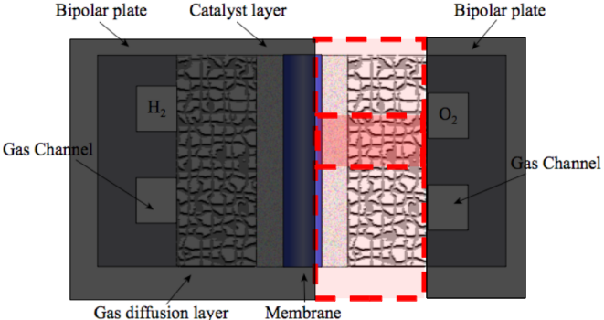
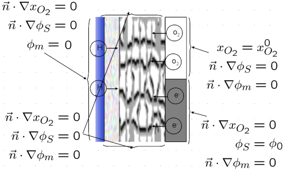
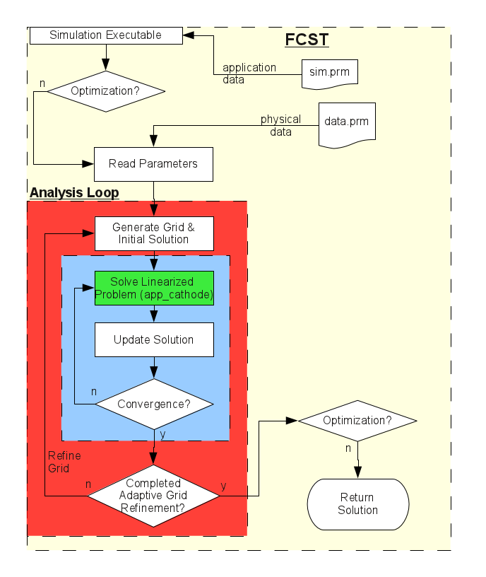
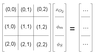
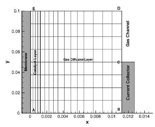
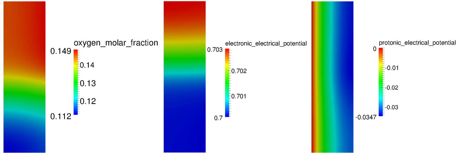
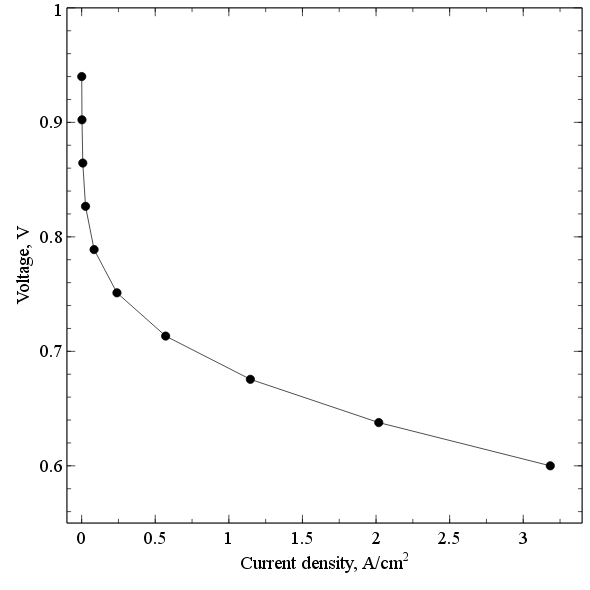
 1.8.5
1.8.5

