- Authors
- The tutorial was developed by Michael Moore and Marc Secanell and later updated by Madhur Bhaiya and P. Mangal
Introduction
This tutorial describes how to develop an application using openFCST. The basic building blocks for creating a fuel cell mathematical model in openFCST are explained using AppCathode application as the template.
AppCathode class implements the polymer electrolyte fuel cell cathode mathematical model proposed in the following publication:
- M. Secanell et al. "Numerical Optimization of Proton Exchange Membrane Fuel Cell Cathode Electrodes",
Electrochimica Acta, 52(7):2668-2682, February 2007.
The data files used to reproduce the results from the publication can be found in folder: /data/cathode//Secanell_EA07_Numerical_Optimization_PEMFC_Cathode_Electrodes. There are several subfolders for analysis, parameteric studies and design cases.
The mathematical model implemented is steady-state, isobaric and isothermal. Oxygen transport is assumed to be diffusion dominated and therefore is represented using Ficks Law. Electronic and protonic transport are governed by Ohms Law. The electrochemical reactions are modelled using Tafel kinetics. Gas diffusion layer and catalyst layer are considered isotropic.
The computational domain is shown in red in the figure below. Due to symmetry of the cell in the vertical direction, the computational domain is reduced to the smaller area encompassed by the red lines by imposing symmetry boundary conditions on the top and bottom boundaries.
The governing equations of the model are written as follows:
\[ R_1(\vec{u}) = \nabla \cdot (c_{total}D^{eff}_{O_2} \nabla x_{O_2} ) = \frac{1}{nF}\nabla\cdot i \]
\[ R_2(\vec{u}) = \nabla \cdot (\sigma^{eff}_{m}\nabla\phi_m) = \nabla \cdot i \]
\[ R_3(\vec{u}) = \nabla \cdot (\sigma^{eff}_{s}\nabla\phi_s) = -\nabla \cdot i \]
where, for the case of a macro-homogeneous catalyst layer,
\[ \nabla \cdot i = A_v i^{ref}_0 \left( \frac{c_{O_2}} {c^{ref}_{O_2}} \right) \mbox{exp} \left( \frac{-\alpha F}{RT}(\phi_s - \phi_m - E_{th}) \right) \]
The solution variables are the protonic potential, \(\phi_m\), the electronic potential, \(\phi_s\) and, the oxygen molar fraction \(x_{O_2}\). Note that the source terms due to current production are only in the catalyst layer, while they are zero in the gas diffusion layer.
The boundary conditions are given by the picture below:
Note that the membrane potential is set to zero at the CCL/membrane interface and that we control the voltage across the cell using the solid phase potential.
The govering equations above are nonlinear. Therefore, a nonlinear solver needs to be used to solve this problem. In OpenFCST, we solve the system of equations using a nonlinear Newton solver. Several nonlinear solvers are provided within the OpenFCST framework and therefore, we do not need to worry about them. You can specify the most appropriate nonlinear solver in the main_app_cathode_analysis.prm file, as follows:
set solver name = Newton3ppC # Linear | NewtonBasic | Newton3ppC | Newton3pp | NewtonLineSearch
When solving a nonlinear problem using a Newton method, an initial solution is needed. In OpenFCST we choose to solve the problem first in a very coarse mesh and then, refine the mesh using a posteriori error estimators. The simulations are intially solved on a relatively coarse grid and it is successively refined after the non-linear system is solved using adaptive refinement. This involves refining the mesh in the areas with the largest error in one of the solution variables between iterations. The routine estimate is used to implement the error estimator for each cell in the domain, for this application. An error estimator developed by Kelly et al. is used to choose the cells needing refinement. The number of refinement leves is defined in the parameter file.
AppCathode and all other applications which you shall develop would need to implemet the linearized form of the govering equations for your problem at the element level. Further routines have already been implemented to loop over the cells in the finite element domain and create the global stiffness matrix and right hand side. The local matrix and right hand side assembly will be implemented in your application in member functions cell_matrix and cell_residual . The global assembly will take place in assemble and residual functions in AppFrame::BlockMatrixApplication which is the parent of all applications in OpenFCST. Based on the above explanation, there are several "levels" within each simulation.
The highest level is the adaptive refinement loop, which will call the Newton solver to solve the non-linear application and then refine the mesh according to the Kelly Error Estimator (provided by deal.II). Again the number of refinement loops is chosen by the user.
The call to the adaptive refinement is made in the simulator builder class. This class is used to set up the simulation at a very high level. It is used to chose a number of key variables which are specified in the main parameter file: the application, solver (there are three Newton solvers with a different line search method) and the solver method (only adaptive refinement is currently implemented). The simulator builder will also define whether we wish to use Dakota to run an optimisation case or parametric study and is where the parameter file with the fuel cell properties, solver properties is selected. Note that to chose the application, solver and solver method, the simulator builder will call the simulator selector class. This class will read the main parameter file and will compare the inputs to a list. If a new application or solver is implemented, it will have to be added to this list. Finally, the call to the simulator builder class is made from the main file.
The next level is a nonlinear application solver which is implemented in the Newton solver classes in FCST. The structure on which these classes are based is contained within AppFrame through the ApplicationCopy class. This will ask the application to solve the linear system, will update the solution according to the chosen line search and repeat until the residual meets the chosen tolerance.
At the lowest level is the system of linearized equations. AppCathode and all other applications are responsible for creating this system of linearized equations and solving it. The Newton solver uses this information to solve the nonlinear problem. The linearization of the governing equations above is given by
\[ -\frac{\partial R_i(\vec{u}^{n-1})}{\partial u_j} (-\delta \vec{u}_j) = -R_i(\vec{u}^{n-1}) \]
where \( n \) is the Newton step. The equations are discretised using finite elements and solved using the Galerkin formulation. The solution is updated and the system is solved again until the desired residual is achieved. This is represented graphically below:
The task of the AppCathode is to create the linearized system of equations above, discretise it and solve it. AppCathode inherits from AppFrame::BlockMatrixApplication. The latter implements a loop over all elements of the computational domain. Therefore, only the local (element level) assembly of the weak form of the governing equations is required. The global system is obtained using routines already implemented. A system matrix is assembled and then it is solved. The equations are stored in OpenFCST, which therefore provides the coefficients for the matrix and RHS. AppFrame provides the data structure for the application (through the BlocMatrixApplication and DoFApplication classes) and the functions to do the assembly. deal.II provides the information about the mesh, the nodes and the finite elements, as well as the solvers for the linear system.
In summary, creating and running a simulation in OpenFCST will consist of creating an application that uses various FCST classes to build a system of local (element level) linear equations that characterizes the fuel cell and solve the global system. These equations are then used by our already implemented routines to assemble the global system (for the whole mesh) and solve the nonlinear problem using a Newton solver. Finally, to increase accuracy the problem is solved in different mesh refinements.
The loops are represented graphically in the figure below:
The linear application contained in the application classes of FCST is represented by the green box, while the Newton solver loop is the blue box. Finally the red represents the adaptive refinement loop. Note that in the flow chart above, the optimisation package implemented in Dakota is not included as it is beyond the scope of this tutorial.
To use the FCST code to create new simulations, the user should only need to create a new linear application. The code is built so that the user should not need to know the deal.II or Appframe libraries in depth, indeed knowledge of the implementation of the Newton solver or the adaptive refinement (both of which are implemented in FCST) is not crucial. A new simulation can be created and run by simply creating a new application so with this in mind the tutorial will start with the header file of an example application, AppCathode, and will explain at a basic level all the components that are required to build the application by examining each line of code in sequence. Then the source file will be examined and provide more depth to the explanation given in the header file.
The simulations are defined using parameter files, simple text files with a .prm file extension that can be read by the FCST code (Note that some parameters can be defined using default values in the code itself, in the
declare_parameters function).
In order to run the simulation, do the following:
- Go to folder /data/cathode//Secanell_EA07_Numerical_Optimization_PEMFC_Cathode_Electrodes/analysis
- In the command terminal type: $../../../../bin/fuel_cell-2d.bin main_app_cathode_analysis.prm
The program will run and return the appropriate results. The main and data parameter files will be explained in the following subsections.The application can be used to solve a cathode with and without an MPL by changing the parameters in the data_app_cathode_parametric.prm file.
The model can also be used to solve an agglomerate catalyst layer model. The governing equations are similar to the ones outlined above, however, the volumetric current density source, i.e. \( \nabla \cdot i \) is obtained as specified in the following article:
-
M. Secanell, K. Karan, A. Suleman and N. Djilali, "Multi-Variable Optimization of PEMFC Cathodes using
an Agglomerate Model ", Electrochimica Acta, 52(22):6318-6337, 2007.
How to modify the parameter file to solve these additional cases will be explain in section The parameter file
A number of different libraries are involved in the simulation, first being the deal.II libraries. These libraries provide the finite elements and linear solvers required to solve the problem. Next are the AppFrame libraries that actually assemble the system of equations and form the basis of the applications that are created in FCST. Finally, the Dakota libraries are used to run optimisation studies and parametric studies.
The commented program
The include file
Here, we will step through the include file,
app_cathode.h, and explain each line of code.The first step is to set the compiler flag that defines this file as the app_cathode class
#ifndef _FUELCELL__APP_CATHODE__H
#define _FUELCELL__APP_CATHODE__H
Next we include all the necessary header files, starting with the general C++ libraries.The first classes to be defined are standard C++ libraries that are used to output data to the screen.
#include "fstream"
#include "iostream"
#include "sstream"
Next are the libraries that form the very core of the simulation, the deal.II libraries. Then the appframe libraries, which are the basis of the applications used in the FCST code. Finally, we will look at the fuel cell specific FCST libraries.
deal.II
The first four are basic components of the FCST code that will be present in all the applications. The parameter_handler class is used to read in the prm files that contain the necessary information to encapsulate a fuel cell simulation.
#include "base/parameter_handler.h"
The function classes are used to create an interface that passes the initial solution to the finite element solver in deal.II. An function object is passed to a deal.II function, VectorTools::interpolate, that will call a
vector_value function from FCST to return the initial solution for the simulation.
#include "base/function_lib.h"
#include "base/function.h"
The quadrature class is used for defining and using
quadrature objects. The main function of these objects is to provide information about the location and weightings of each quadrature point in a cell.
#include "base/quadrature_lib.h"
The next block of classes are related to the
solvers that will be used to solve the system of equations.
#include "lac/block_vector.h"
#include "lac/full_matrix.h"
#include "lac/solver_cg.h"
#include "lac/solver_gmres.h"
#include "lac/precondition.h"
#include "lac/precondition_block.h"
#include "lac/block_matrix_array.h"
#include "lac/filtered_matrix.h"
#include "lac/sparse_ilu.h"
#include "lac/sparse_direct.h"
Next are the
grid classes, with one for generating grid, two for looping over cell or faces and another to handle boundary conditions.
#include "grid/grid_generator.h"
#include "grid/tria_accessor.h"
#include "grid/tria_iterator.h"
#include "grid/tria_boundary_lib.h"
The
fe values class is used to store information about the finite elements that are used to discretise the equations.
#include "fe/fe_values.h"
The
numerics classes are used to define convenient objects that are used to store information in a manner more suited to scientific computing. They include vector and matrix classes which are used widely in FCST. Also included is the error_estimator class, which is used for grid refinement.
#include "numerics/vectors.h"
#include "numerics/matrices.h"
#include "numerics/error_estimator.h"
Finally, the deal.II library includes boost as one of its contributing libraries. Here we use the boost shared_pointers instead of C++ pointers because they are more robust in terms of memory leaks.
#include "boost/shared_ptr.hpp"
Appframe
Next is the appframe libraries, which are used to build the system of equations. The block_matrix_application class is one of the parent classes of the applications used in FCST. All applications inherit from block_matrix_application. optimization_block_matrix_application which inherits from block_matrix_application and in turn applications inherit directly from it. It allows for the optimisation of simulations using the Dakota libaries.
The last two classes used from appframe, are the appshop classes used to assemble the right and left hand side of our equations.
FCST
The FCST classes are those that are specific to the generation of a fuel cell simulation. The first is Solver_utils which contains a few functions that used by the solvers to check and modify the diagonal entries of the assembled matrix.
Next is the geometries class which defines the dimensions of the cell, generates the grid for each layer and contains the material id and boundary ids.
The next three classes to be defined are the constants class, which contains universal constants such as Faradays constant or the gas constant. The operating conditions class defines variables such as the operating temperature of the cell, the pressure at the cathode or the molar fraction of hydrogen at the anode and the system management class contains all the equations, variable names used in FCST, and also used for coupling the equations. Depending on the simulations, relevant equations and variables are accessed.
Next are two classes that describe the gases used in the fuel cell and how they interact. The first contains the properties about a number of different gases, for example the viscosity of oxygen or critical temperature of nitrogen. Also described are hydrogen and water vapour. The second describes their interaction. The class will take two gases and return the diffusion coefficient according to Chapman Enskog theory for gas diffusion and Wilke Chang or Hans Bartels Interpolation for liquid diffusion.
OpenFCST contains classes that implment the weak form of many partial differential equations that govern the physical processes in a fuel cell. For example, classes exist to implement the weak form of Fick's law of diffusion, Ohm's law, the Navier-Stoke equations, etc. All this classes are stored inside the #Equation namespace in FCST.
In our application, we need Fick's law, Ohm's law for that electron and protons and a source term for the electrochemical reaction. This objects are included in our application here.
A fuel cell is made of many composite materials for which effective properties need to be obtained. OpenFCST contains a library of layers for fuel cells under namespace #Layers. The layers are made of different materials and are used to compute the coefficients for the governing equations implemented in the classes above. Layer classes will return information about the effective transport properties of species through each layer, e.g. oxygen diffusion, protonic conductivity, permeabilities etc. The catalyst layers also provide the interface to the kinetics class, which handle the electrochemical reactions in the cell.
Because OpenFCST code relies heavily on the deal.II libraries, the deal.II namespace is used in most of the header files. This saves from prefixing all calls to deal.II functions and member variables with deal.II.
The Member Function Declaration
FCST function and member variables use one of the
FuelCell namespaces. There are two main namespaces,
FuelCell and
FuelCellShop.
FuelCellShop is the container for the data classes while
FuelCell contains the applications, geometries and intial solutions. The main namespace that is used is the
FuelCell::Application, the container for all the applications that have been developed for the FCST code.
Application namespace is used for all applications, i.e. all the routines that implement the linear system to be solved using a Newton solver.
For any application, the first that needs to be declared is a constructor and a destructor. When creating an application, the constructor will create an object of type application data (
AppFrame::ApplicationData). This is a structure that will handle the general data for the application.
AppCathode ( boost::shared_ptr<AppFrame::ApplicationData> data =
boost::shared_ptr<AppFrame::ApplicationData> () );
The class destructor will delete any pointers that have not been used by the class. *
All applications have a delcare_parameters function. This function is used to specify the data that is expected from the input file and default data to be used in case the input file does not contain any information for that variable. The data is stored in the ParameterHandler object which is an object in the nonlinear application.
virtual void declare_parameters ( ParameterHandler& param );
All applications that are used for parameteric and optimization studies with Dakota need the function set_parameters. This function is called by the optimization loop in order to set the values in the ParameterHandler to the new design parameters.
Since ParameterHandler depends on the problem we are solving, set_parameters() is set at the most inner loop of the application.
virtual void set_parameters ( const std::vector<std::string>& name_dvar,
const std::vector<double>& value_dvar,
ParameterHandler& param );
All applications have a routine initialize. This routine is used to read from ParameterHandler object the values for all the data necessary to setup the application problem to be solved. Note that declare_parameters simply specifies the values that will be read from file. In initialize, the values from the input file are actually read and stored inside the application for later use.
virtual void initialize ( ParameterHandler& param );
This routine is called by initialize and it is simply used to initialize data unique to the application.
void _initialize ( ParameterHandler& param );
Initilize also creates the computational domain. To do so it will call this routine which determines whether reading from a grid file or creating new mesh
void initialize_grid ( ParameterHandler& param );
This member function is used to create the initial solution for our problem
All application need a member function, cell_matrix, that generates the element wise finite element matrix for the system of equations that is solved. Here we loop over the quadrature points and over degrees of freedom in order to compute the matrix for the cell This routine depends on the problem at hand and is called by assemble() in DoF_Handler class The matrix to be assembled in our case is of the form:
\[ \begin{array}{l} M(i,j).block(0) = \int_{\Omega} a \nabla \phi_i \nabla \phi_j d\Omega + \int_{\Omega} \phi_i \frac{\partial f}{\partial u_0}\Big|_n \phi_j d\Omega \\ M(i,j).block(1) = \int_{\Omega} \phi_i \frac{\partial f}{\partial u_1}\Big|_n \phi_j d\Omega \\ M(i,j).block(2) = \int_{\Omega} \phi_i \frac{\partial f}{\partial u_2}\Big|_n \phi_j d\Omega \end{array} \]
This matrix will be assembled using Equation objects as discussed later.
All application need a member function, cell_residual, that generates the element wise finite element right hand side for the system of equations that is solved. Integration of the rhs of the equations. Here we loop over the quadrature points and over degrees of freedom in order to compute the right hand side for each cell This routine depends on the problem at hand and is called by residual() in DoF_Handler class. Note that this function is called residual because in the case of nonlinear systems the rhs is equivalent to the residual
If Dirichlet boundary conditions need to be applied to the problem, the application will have to implement this member function, i.e. dirichlet_bc. This member function is used to set dirichlet boundary conditions. This function is application specific and it only computes the boundary_value values that are used to constraint the linear system of equations that is being solved
virtual void dirichlet_bc ( std::map<unsigned int, double>& boundary_values ) const;
All applications need a member function to solve the global system of equations.
If we want to use adaptive refinement, we need to estimate the error per cell. This value will be used to refine the mesh as needed.
Post-processing. This routine is called at post-processing and it is used to evaluate a functional such as the current density
This routine is used to create the output file. A base member function already exists, but in AppCathode we will reimplement it so that the right labels are outputed and so that I can compute and output the source terms.
virtual void data_out ( const std::string &basename,
The Member Variables
In this section we will look at the member variables that are used in this application so the basis of the simulation can be understood. This are usually protected:
The first variable is system_management and it is used to store all information related to the system of equations that is being solved such as variable_names, equation_names and couplings between equations.
The second member variable is the operating conditions object that was passed to the initial solution object and explained in more detail in the previous section.
Next is the grid object which is derived from the
geometries class. As was previously mentioned this object will define the dimensions of the cell, generates the grid for each layer and contains the material and boundary ids.
Instead of creating an object, a boost pointer of the base class is used. This is done so that I can select the appropriate child at run-time after checking the input file.
boost::shared_ptr< FuelCellShop::Geometry::GridBase<dim> > grid;
The cathode contains oxygen, nitrogen and water vapour, so we need to create an object for each gas in order to compute viscosity, density, etc.
Next the cathode gas diffusion layer (CGDL) and cathode catalyst layer (CCL) are created. Again a pointer is used to the base class for each type of layer. We will then select the appropriate CGDL / CCL once we have read the input file. Using a pointer allows us to code everything independently of the layer we want to use. This allows users to develop their own layers. By making them a child of the base class, for example FuelCellShop::Layer::GasDiffusionLayer<dim>, the application will run for your new layer without any modification. For info on how to create your own layer, please consult the documentation on the base layer clases
boost::shared_ptr<FuelCellShop::Layer::GasDiffusionLayer<dim> > CGDL;
boost::shared_ptr<FuelCellShop::Layer::MicroPorousLayer<dim> > CMPL;
boost::shared_ptr<FuelCellShop::Layer::CatalystLayer<dim> > CCL;
OpenFCST contains a database of materials and layers, but also a database that contains the discrtization of most physical equations relavant to fuel cells. Therefore, we will create an object of the physical processes that are relevant to the cathode.
For the cathode we need an Ohm's law equation for electrons, a Fick's law equation for oxygen and an Ohm's law equation for protons. We also need a source term for the reaction rates.
The equation class used to assemble the cell matrix for electron transport is
The equation class used to assemble the cell matrix for Fick's mass transport.
Equation class used to assemble the cell matrix for proton transport
The Equation class to assemble the cell matrix and cell_residual for the reaction source terms is the last object. After that, we finish the declaration of the class and the namespaces in the
app_cathode.h file.
};
}
}
#endif //_FUELCELL__APP_CATHODE_H
Source File
The Member Functions
All source files need to include the .h file. Therefore, the first line in our code is
Since all member functions are in namespace FuelCell::Application is useful to define a shortcut. Also, AppFrame functions are used all the time, so we use using namespace AppFrame so that we do not need to specify the namespace.
namespace NAME = FuelCell::Application;
using namespace AppFrame;
Now, we are ready to start the implementation of all the member functions in AppCathode.
Each application is based on the application base class in appframe (
AppFrame::ApplicationBase), in particular the
OptimizationBlockMatrixApplication class (
AppFrame::OptimizationBlockMatrixApplication). This class is the last in a series of inherited classes starting with ApplicationBase that includes
DoFApplication (
AppFrame::DoFApplication) and BlockMatrixApplication (
AppFrame::BlockMatrixApplication). The
DoFApplication contains a handler for the degrees of freedom,
Triangulation and the mesh. BlockMatrixApplication handles the matrices and the assembling of the linear systems of equations.
OptimizationBlockMatrixApplication was then added by the OpenFCST developers to handle sensitivity analysis. As such all applications are inherited from OptimizationBlockMatrix.
AppCathode constructor will therefore initialize
OptimizationBlockMatrixApplication. Also, all equation classes need to be created during the constructor. Finally, we output a line to the terminal stating that this application has been created.
template <int dim>
NAME::AppCathode<dim>::AppCathode(boost::shared_ptr<AppFrame::ApplicationData> data)
:
ficks_transport_equation(system_management,&oxygen, &nitrogen),
electron_transport_equation(system_management),
proton_transport_equation(system_management),
reaction_source(system_management)
{
deallog <<
"->FuelCell::Application::AppCathode_test-" <<
dim <<
"d"<<std::endl;
}
The destructor for AppCathode does not need to remove any extra pointers since boost pointers have their own memory management strategy.
template <int dim>
NAME::AppCathode<dim>::~AppCathode()
{}
Now that the application is created, the next step is to provide the required information to run a simulation. There are three functions that are used to do this. The first is the
declare_parameters function. The application needs to declare the parameters it needs from file, but all other objects used by the applicaiton also need to do the same thing. Therefore, declare_parametes contains a call to declare_parameter for all the Materials, Layers and Equation classes. Note that for the Layers and Geometry, a static function is called. The name provided in the call, e.g. "Cathode gas diffusion layer", is the name of the section in the input file where the information need to be provided.
template <int dim>
void
NAME::AppCathode<dim>::declare_parameters(ParameterHandler& param)
{
system_management.declare_parameters(param);
OC.declare_parameters(param);
electron_transport_equation.declare_parameters(param);
proton_transport_equation.declare_parameters(param);
ficks_transport_equation.declare_parameters(param);
reaction_source.declare_parameters(param);
}
Each one of the declare_parameter calls tells the application what parameters might be passed to it by the .prm file. In the operating conditions class for example, 'entries' such as the temperature of the cell, the cathode pressure or the RH of the cathode are created by the function and are given a default value. The function also tells the application what type of a value to expect, double, int, bool etc. and optionally a short description of the parameter.For example, the OperatingConditions
declare_parameters code looks as follows:
void
{
param.enter_subsection("Fuel cell* data");
{
param.enter_subsection("Operating conditions");
{
param.declare_entry ("Temperature cell",
"353",
Patterns::Double());
param.declare_entry ("Cathode pressure",
"101325",
Patterns::Double(),
"Pressure at the cathode channel in Pa");
param.declare_entry ("Cathode relative humidity",
"0.7",
Patterns::Double(),
"Relative humidity (fraction) in the cathode channel");
param.declare_entry ("Anode pressure",
"101325",
Patterns::Double(),
"Pressure at the anode channel in Pa");
param.declare_entry ("Anode relative humidity",
"0.7",
Patterns::Double(),
"Relative humidity (fraction) in the anode channel");
param.declare_entry ("Voltage cell",
"0.6",
Patterns::Double());
param.declare_entry("Voltage drop in the anode",
"0.015",
Patterns::Double());
param.declare_entry ("Open circuit voltage",
"1.23",
Patterns::Double());
}
param.leave_subsection();
}
param.leave_subsection();
}
The prm file is a file containing a list of these parameters as specified by all the
declare_parameters functions. It is divided into sections and subsections each having their own label as defined by the
declare_parameters functions. For example the operating conditions parameters are found in the "Operating conditions" subsection under the "Fuel cell data" subsection. This section from the prm file is given below:
subsection Fuel cell data
subsection Operating conditions
set Temperature cell = 383 #[
K]
set Cathode pressure = 101265 #[Pa] (1 atm)
set Cathode relative humidity = 0.6
set Voltage cell = 0.822 ## Convergence up to 0.66V
end
end
Note that not all the entries declared in the source code are found in the prm file, for example "Anode
relative humidity". In this case the default value will be used. Also when defining a parameter, the units should be included. For example the entry for the cell temperature should be "Temperature cell [K]".
Users do not usually need to look at the code to see the parameters that are declared, the DOxygen documentation, under declare_parameters, will explain the values declared.
If an optimisation case is being run, then the application will need to know the parameters that are to be optimised. This is done using the
set_parameters function. Here the function stores the names of the parameters to be optimised, in the vector of strings
name_dvar, and it's values, in the vector of doubles
value_dvar. These are then handled by the optimization_block_matrix_application class. In the application, the function simply calls the
set_parameters functions of the relevant classes:
template <int dim>
void
NAME::AppCathode<dim>::set_parameters(const std::vector<std::string>& name_dvar,
const std::vector<double>& value_dvar,
ParameterHandler& param)
{
OC.set_parameters(name_dvar, value_dvar, param);
design_var = name_dvar;
design_var_value = value_dvar;
}
The initialise function is the final function in setting up the simulation. It actually parses the prm file, extracts the required values and assigns them to the relevant variables. Again the application function calls the functions of the contributing classes.
In initialize, the ParameterHandler object param already contains the information from the input file. Now this information needs to be distributed to all object in the application.
First, we initialize system_management and operating_conditions (OC):
template <int dim>
void
NAME::AppCathode<dim>::_initialize(ParameterHandler& param)
{
system_management.initialize(param);
OC.initialize(param);
}
The contributing classes initialise functions actually extract and set the required values, for example, the call
OC.initialize(param); will run the following function:
void
{
param.enter_subsection("Fuel cell data");
{
param.enter_subsection("Operating conditions");
{
T_cell = param.get_double(
"Temperature cell");
V_cell = param.get_double(
"Voltage cell");
p_c = param.get_double(
"Cathode pressure");
RH_c = param.get_double(
"Cathode relative humidity");
p_a = param.get_double(
"Anode pressure");
RH_a = param.get_double(
"Anode relative humidity");
V_cell = param.get_double(
"Voltage cell");
dV_a = param.get_double(
"Voltage drop in the anode");
OCV = param.get_double(
"Open circuit voltage");
{
param.set(
"Open circuit voltage",
OCV);
}
}
param.leave_subsection();
}
param.leave_subsection();
}
The next step is to set up the grid. For this, we call the #initialize_grid function which will be implemented next. This member function will read in and set variables such as the number of divisions in the CGDL and CCL, the material and boundary IDs and the physical dimensions and then generate the mesh and store it the object this->tr.
this->initialize_grid(param);
The initialise function in the application actually does more than set up the parameters for the simulation, it also initialises the Materials, Layers and Equation objects and also the kinetics class for cathode catalyst layer. In this case, we first create a vector with all the gases that will exist in the layers.
Next, we call create_GasDiffusionLayer("Cathode gas diffusion layer",param) This function reads the parameter file section Fuel Cell Data > Cathode gas diffusion layer, reads the type of GDL that we would like to use, and then initializes the pointer CGDL to the appropriate GasDiffusionLayer child. In this case, DesignFibrousGDL as we will see when discussing the parameter file.
One the layer has been initialized, we "fill" the layer with the gases using CGDL->set_gases_and_compute(gases, OC.get_pc_atm (), OC.get_T()). This routine is used to store the gases, the temperature and the pressure in the layer and to compute the diffusion coefficients.
The MicroPorousLayer and CatalystLayer objects are initialized using the same method.
std::vector< FuelCellShop::Material::PureGas * > gases;
gases.push_back(&oxygen);
gases.push_back(&nitrogen);
CGDL->set_gases_and_compute(gases, OC.get_pc_atm (), OC.get_T());
CMPL->set_gases_and_compute(gases, OC.get_pc_atm (), OC.get_T());
CCL->set_gases_and_compute (gases, OC.get_pc_atm (), OC.get_T());
For the CatalystLayer object, in addition to specifying the type of gas inside the layer, we also need to specify the reactions that we are interested in solvign for since the catalyst layer class contains a kinetics objects which will compute the reaction rates for different reactions. In order to compute the reactions, we need to know the overpotential, temperature and pressure. Every time we call the cell_matrix and cell_residual function, we pass the solution (which will contain the oxygen molar fraction and the two potentials) to the kinetics class. However the kinetics class expects that the temperature and pressure are solution variables (i.e.that it is set at each quadrature point for each cell).
(OC.get_pc_Pa(), total_pressure) and
(OC.get_T(), temperature_of_REV) are used to specify that these variables are constant and should take the value provided as the first argument.
std::string name = "ORR";
CCL->set_reaction_kinetics(name);
Once the layers have been initialized, it is time to initialize the Equation objects.
Before initializing the objects, we set the kinetics in the reaction source term object. Next, we allow all Equation object to read all their parameters from file: *
reaction_source.set_cathode_kinetics(CCL->get_kinetics());
electron_transport_equation.initialize(param);
proton_transport_equation.initialize(param);
ficks_transport_equation.initialize(param);
reaction_source.initialize(param);
Next is to prepare the matrix that will contain our system of equations. This involves telling the application how the equations are coupled, i.e. how one solution variable affects the other equations. The blocks for our three equation system are visualised below:
If the variable is not in the equation then this block will contain zeros. To save memory,
AppFrame will not store this block: if, for example, the membrane potential was not present in the third equation for the solid phase potential then there would only be 8 blocks. In this case the system of equations is fulled coupled as the source term for each equation contains each of the solution variables. To get the information about coupling, a vector "tmp" is created, push_back function is used to get internal cell couplings for all three equations then the couplings are adjusted after including the source term. Finally the couplings are generated in system management.
std::vector<couplings_map> tmp;
tmp.push_back(ficks_transport_equation.get_internal_cell_couplings() );
tmp.push_back(proton_transport_equation.get_internal_cell_couplings() );
tmp.push_back(electron_transport_equation.get_internal_cell_couplings() );
reaction_source.adjust_internal_cell_couplings(tmp);
system_management.make_cell_couplings(tmp);
Given that the grid has now been set up, we can now give it the information about the degrees of freedom (dof) to be associated with each cell. This information is stored using a deal.II object called
DoFHandler that will look at the type of finite elements that the simulation is using and allocate space for the dof. The finite elements we are using are defined in the parameter file, under the section Discretisation > Element. In the test case, we are using three first order elements which are defined using:
FESystem[FE_Q(1)^3]. If second order elements are required, then we would use:
FESystem[FE_Q(2)^3]. To use different elements for an equation, for example first order for the first equation and second order for the other two, we would write
FESystem[FE_Q(1)]-FESystem[FE_Q(2)^2]. This is implemented in the deal.II
FiniteElement classes.
The
remesh_dofs() will also assign indices to the cells and faces that will be used later in the error estimator.The next step is to initialise the matrix that will store the system of equations.
This is all. Finally, we simply call some routines that are used to print information to screen in order to make sure we have initialized our layers correct.
CCL->print_layer_properties ();
}
The initialise function above is used to initialise the FCST classes, however the FCST applications are built on a hierarchy of appframe classes that also have to be initialised. For that reason, the main program doesn't call the
_initialise function described above, but
intialise instead. This function will call the
_initialise function but will also call the initialise function of the applications parent class,
OptimizationBlockMatrixApplication . This has its own initialise function that will initialise its classes, and also call the initialise function of its parent class,
BlockMatrixApplication . This continues on to
DoFApplication and
ApplicationBase .
template <int dim>
void
{
_initialize(param);
}
The grid can be initialized in two ways. If we have a mesh from a file (i.e. read_grid_from_file == true) or we have a mesh from a previous simulation (this->read_in_initial_solution == true), e.g. if running a polarization curve, then, the previous mesh can be read from file and used to initialize the mesh.
Otherwise, use our boost::shared_ptr< FuelCellShop::Geometry::GridBase<dim> > object to generate the mesh using grid->generate_grid(*this->tr);
template <int dim>
void
NAME::AppCathode<dim>::initialize_grid(ParameterHandler& param)
{
AssertThrow (( (grid->get_mesh_type()).compare("Cathode") == 0 || (grid->get_mesh_type()).compare("CathodeMPL") == 0 || (grid->get_mesh_type()).compare("GridExternal") == 0),
ExcMessage("Only GridExternal, Cathode and CathodeMPL meshes are permitted for AppCathode. Check entry Type of mesh in subsection Grid generation in the parameter file"));
bool read_grid_from_file = grid->read_from_file;
if (this->read_in_initial_solution || read_grid_from_file)
{
std::ifstream grid_file("._mesh_to_be_transfered.msh");
if(!grid_file.fail())
{
deallog << "Reading grid from file" << std::endl;
GridIn<dim> grid_in;
grid_in.attach_triangulation(*this->tr);
grid_in.read_msh(grid_file);
grid_file.close();
read_grid_from_file = true;
}
else
{
deallog << "Grid file not available for reading" << std::endl;
read_grid_from_file = false;
this->read_in_initial_solution = false;
}
}
if(!read_grid_from_file)
{
deallog << "Generating new grid" << std::endl;
grid->generate_grid(*this->tr);
}
}
To actually generate a grid using deal.ii, an object of type
triangulation is used (here its pointed to by
this->tr). This is a deal.II object that contains information about the geometric and topological properties of a mesh, for example the location of vertices of the cell and how they are connected. The same triangulation object is also used while reading grid from file.The geometries class contains a number of methods for generating a grid depending on whether we are running a cathode, pemfc, anode with MPL etc. simulation. In this case we are running a simple cathode catalyst layer with GDL/MPL simulation.
generate_grid will take the dimensions of the fuel cell and divide it up into a mesh depending on how many horizontal and vertical divisions we set. Then it will loop over all cells and their vertices and assign material and boundary ids according to how far a vertex is from the origin in the horizontal direction. Optionally, the grid will then be refined once.
The last part of the setting up the simulation involves providing information about the initial solution to the nonlinear solver. This is done with the
init_solution function.
template <int dim>
void
{
The operating molar fraction of oxygen in the channel and voltage cell are first read from operating_conditions class.
double x_o2 = OC.get_x_o2();
double V_cell = - OC.get_V();
The vector
dst has to be initialized to the initial solution. The first step is to resize the
dst vector to the size of the solution vector.
dst.reinit(this->block_info.global);
To input the initial solution to the solution vector, two functions are created called function_map and component_mask. The former is used to relate a material ID to a function type. For example, for the catalyst layer material id, the oxygen concentration should be \( c_0 \).
std::map<types::material_id, const Function<dim>* > function_map;
std::vector<bool> component_mask(3, false);
We will use a piece-wise constant function as the initial solution. The solution will be constant within each layer and will change in value between layers. Therefore, we need the functions that will provide the value of the solution at each point in the mesh. These functions are defined below and are given to the function_map such that the mole fraction in the GDL is the same as in the channel and MPL and catalyst layer contain half and a quarter of the oxygen respectively. function_map is used to identify the layer via material id.
const ConstantFunction<dim> f_xo2_GDL(x_o2, 3);
const ConstantFunction<dim> f_xo2_MPL(x_o2/2.0, 3);
const ConstantFunction<dim> f_xo2_CL(x_o2/4.0, 3);
function_map[CGDL->get_material_id()] = &f_xo2_GDL;
function_map[CMPL->get_material_id()] = &f_xo2_MPL;
function_map[CCL->get_material_id()] = &f_xo2_CL;
Next, component_mask is used to identify the solution variable name for which the initial solution is being set up. Finally the deal.II function
interpolate is used to distribute the initial solution on the cell.
std::vector< std::string > solution_names( system_management.get_solution_names () );
for (unsigned int i = 0; i<solution_names.size(); i++)
{
if (solution_names[i] == "oxygen_molar_fraction")
component_mask[i] = true;
else
component_mask[i] = false;
}
VectorTools::interpolate( dst,
this->mapping,
this->dof,
function_map,
component_mask );
We repeat the same process for the electrolyte and electrical potential:
const ConstantFunction<dim> f_fp(0.0, 3);
function_map[CGDL->get_material_id()] = &f_fp;
function_map[CMPL->get_material_id()] = &f_fp;
function_map[CCL->get_material_id()] = &f_fp;
for (unsigned int i = 0; i<solution_names.size(); i++)
{
if (solution_names[i] == "protonic_electrical_potential")
component_mask[i] = true;
else
component_mask[i] = false;
}
VectorTools::interpolate( dst,
this->mapping,
this->dof,
function_map,
component_mask );
const ConstantFunction<dim> f_fe(V_cell, 3);
function_map[CGDL->get_material_id()] = &f_fe;
function_map[CMPL->get_material_id()] = &f_fe;
function_map[CCL->get_material_id()] = &f_fe;
for (unsigned int i = 0; i<solution_names.size(); i++)
{
if (solution_names[i] == "electronic_electrical_potential")
component_mask[i] = true;
else
component_mask[i] = false;
}
VectorTools::interpolate( dst,
this->mapping,
this->dof,
function_map,
component_mask );
}
Please note that our initial solution meets the Dirichlet boundary conditions. This is necessary when setting up the problem.
The simulation has now been set up so we can start to work on the member functions that are used to assemble the local (element-wise) matrix and residual (right hand side).
The two most important functions in the application are the
cell_matrix and
cell_residual functions. The functions provide the coefficients for the left and right hand side of our linearised system of equations respectively ( \(\frac{dR(u,p)}{du}(-\delta u) = R(u,p)\)).
We will start with the
cell_matrix function which implements the integration of the local bilinear form. Here we loop over the quadrature points and over degrees of freedom in order to compute the matrix for the cell. This routine depends on the problem at hand and is called in
assemble in BlockMatrixApplication class.
In this case, the matrix to be assembled is given below:
\begin{eqnarray} M(i,j).block(0) & = & \int_{\Omega} a \nabla \phi_i \nabla \phi_j d\Omega + \int_{\Omega} \phi_i \frac{\partial f}{\partial u_0}\Big|_n \phi_j d\Omega \quad \qquad & M(i,j).block(1) & = & \int_{\Omega} \phi_i \frac{\partial f}{\partial u_1}\Big|_n \phi_j d\Omega & M(i,j).block(2) & = & \int_{\Omega} \phi_i \frac{\partial f}{\partial u_2}\Big|_n \phi_j d\Omega \\ M(i,j).block(3) & = & \int_{\Omega} \phi_i \frac{\partial f}{\partial u_0}\Big|_n \phi_j d\Omega & M(i,j).block(4) & = & \int_{\Omega} a \nabla \phi_i \nabla \phi_j d\Omega + \int_{\Omega} \phi_i \frac{\partial f}{\partial u_1}\Big|_n \phi_j d\Omega \quad \qquad & M(i,j).block(5) & = & \int_{\Omega} \phi_i \frac{\partial f}{\partial u_2}\Big|_n \phi_j d\Omega \\ M(i,j).block(6) & = & \int_{\Omega} \phi_i \frac{\partial f}{\partial u_0}\Big|_n \phi_j d\Omega & M(i,j).block(7) & = & \int_{\Omega} \phi_i \frac{\partial f}{\partial u_1}\Big|_n \phi_j d\Omega& M(i,j).block(8) & = & \int_{\Omega} a \nabla \phi_i \nabla \phi_j d\Omega + \int_{\Omega} \phi_i \frac{\partial f}{\partial u_2}\Big|_n \phi_j d\Omega \end{eqnarray}
OpenFCST already contains many equation classes which are used to assemble the local cell matrices. Therefore, assembling the matrices is extremely simple. Simply call the Equation classes you want to solve!
cell_matrix receives a MatrixVector object containing a vector of local matrices corresponding to all the non-zero matrices in the global matrix such that cell_matrices[0] corresponds to M(i,j).block(0), and a CellInfo object that
template <int dim>
void
NAME::AppCathode<dim>::cell_matrix(
MatrixVector& cell_matrices,
{
In this case, we solve a different set of equations for each layer. In the gas diffusion layer, we solve for Fick's law of diffusion and electron transport. Therefore, we can ask our Equation classes to assemble the local matrices for GDL cells using the information provided by the CGDL class.
A particular layer is identified through its material id for any particular cell. The information of material id is accessed using the member function material_id() in the
info object.
Equation classes such as
ficks_transport_equation,
electron_transport_equation,
proton_transport_equation and
reaction_source have an inbuilt function
assemble_cell_matrix which assembles the local matrix and passes the local matrix to the MatrixVector which is a vector of local matrices, it assembles the local matrices and make them global. The call to
assemble_cell_matrix will return M(i,j).block(0) filled based on the properties of the cell and the CGDL.
if (CGDL->belongs_to_material(info.cell->material_id()))
{
ficks_transport_equation.assemble_cell_matrix(cell_matrices, info, CGDL.get());
electron_transport_equation.assemble_cell_matrix(cell_matrices, info, CGDL.get());
}
The same process can be applied the MPL:
else if (CMPL->belongs_to_material(info.cell->material_id()))
{
ficks_transport_equation.assemble_cell_matrix(cell_matrices, info, CMPL.get());
electron_transport_equation.assemble_cell_matrix(cell_matrices, info, CMPL.get());
}
For the catalyst layer, we wish to solve not only for oxygen and electron transport but also for proton transport and for the reaction terms. Therefore, all four Equation objects are called in order to provide the required information in cell_matrices.
else if (CCL->belongs_to_material(info.cell->material_id()))
{
ficks_transport_equation.assemble_cell_matrix(cell_matrices, info, CCL.get());
electron_transport_equation.assemble_cell_matrix(cell_matrices, info, CCL.get());
proton_transport_equation.assemble_cell_matrix(cell_matrices, info, CCL.get());
reaction_source.assemble_cell_matrix(cell_matrices, info, CCL.get());
}
Finally, if the mesh contains cells with a material ID that does not correspond to any of the layers defined in the application, we will ask the program to provide an error message:
else
{
deallog<<"Material id: " <<info.cell->material_id()<<" does not correspond to any layer"<<std::endl;
}
}
Using the process specified above, local cell matrices are formed for all three layers and equations.
This completes the
cell_matrix function. We can now move onto the
cell_residual and the right hand side (RHS).
The
cell_residual function works similarly to the
cell_matrix member function. The main difference is that in constructing the RHS we are not assembling a matrix, but a vector, which is why
cell_vector is passed in the
cell_residual function call.
The vector were are constructing is given by:
\[ R(i),block(i) = \int_{\Omega} \phi_j a (\nabla u)^n d\Omega + \int_{\Omega} \phi_j f(u^n) d\Omega \]
In our case this can be written as:
\begin{eqnarray} R(i),block(0) & = & \int_{\Omega} \phi_j D_{O_2} (\nabla x_{O_2})^n d\Omega + \int_{\Omega} \phi_j \left( \frac{i(u^n)}{4F} \right) d\Omega \\ R(i),block(1) & = & \int_{\Omega} \phi_j \sigma_m (\nabla \phi_m)^n d\Omega + \int_{\Omega} \phi_j \left( \frac{i(u^n)}{F} \right) d\Omega \\ R(i),block(2) & = & \int_{\Omega} \phi_j \sigma_s (\nabla \phi_m)^n d\Omega + \int_{\Omega} \phi_j \left( \frac{i(u^n)}{-F} \right) d\Omega \end{eqnarray}
where \( u^n \) is the solution at the \( n \) iteration in the Newton loop.
cell_residual takes two arguments, a BlockVector that should be initialized to the local right hand side, i.e. element-wise right hand side, and a CellInfo object that contains information regarding the cell finite element, material id, boundary id and the solution at the quadrature points in the cell. This information is used to setup the right hand side.
As in cell_matrix, we first check at which material the cell belongs to and, based on its material id, we use the appropriate Equation class to assemble the right hand side. In this case, this is done by calling the member function assemble_cell_residual.
template <int dim>
void
{
Assert (cell_vector.n_blocks() == this->element->n_blocks(),
ExcDimensionMismatch (cell_vector.n_blocks(), this->element->n_blocks()));
if (CGDL->belongs_to_material(info.cell->material_id()))
{
ficks_transport_equation.assemble_cell_residual(cell_vector, info, CGDL.get());
electron_transport_equation.assemble_cell_residual(cell_vector, info, CGDL.get());
}
else if (CMPL->belongs_to_material(info.cell->material_id()))
{
ficks_transport_equation.assemble_cell_residual(cell_vector, info, CMPL.get());
electron_transport_equation.assemble_cell_residual(cell_vector, info, CMPL.get());
}
else if (CCL->belongs_to_material(info.cell->material_id()))
{
ficks_transport_equation.assemble_cell_residual(cell_vector, info, CCL.get());
electron_transport_equation.assemble_cell_residual(cell_vector, info, CCL.get());
proton_transport_equation.assemble_cell_residual(cell_vector, info, CCL.get());
reaction_source.assemble_cell_residual(cell_vector, info, CCL.get());
}
else
{
deallog<<"Material id: " <<info.cell->material_id()<<" does not correspond to any layer"<<std::endl;
}
}
Next, we need to define the boundary conditions for the three solution variables. Note that since we are solving a linearized system, the boundary conditions are not for the solution variables oxygen mole fraction, electrical and proton potential, but for their variation, i.e. \( \delta u \) instead of \( u \). Therefore, the variation of each boundary conditon of the nonlinear problem needs to be implemented here.
Dirichlet boundary conditions on the solution variables have a variation of zero, i.e. if the initial solution satisfies the boundary conditions, the Dirichlet boundary conditions on the variations are that the variation should be zero.
Imposing a zero Dirichlet boundary condition is done by the
dirichlet_bc function. This function fills a std::map named boundary_values with an unsigned int representing the degree of freedom and the Dirichlet value of the boundary condition. In this case, all Dirichlet boundaries will have a zero value.
template <int dim>
void
NAME::AppCathode<dim>::dirichlet_bc(std::map<unsigned int, double>& boundary_values) const
{
We will analyze one boundary at a time. The boundaries are identified using boundary ids, which are integer numbers that are specified when constructing the mesh. Boundary ids are stored in the grid class and are accessed using the
get_boundary_id function by passing a string that identifies the requested boundary. In the code below, we want to apply a boundary condition at the membrane/catalyst layer interface.
The boundary values can be applied to any of the solution variables. For the case of the membrane/catalyst layer interface we would like to apply a Dirichlet boundary conditon to the electrolyte potential, i.e. the Protonic electrical potential variable, since the potential there is specified. The oxygem mole fraction and electrical potential are not specified at that interface. The
comp_mask vector is used to denote whether a solution variable should be specified or not. Therefore, we set the comp_mask corresponding to the proton potential to true, while the others are set to false.We have now identified the variable we want to apply the boundary conditions to and we now need to fill out the boundary_values. To setup the values at each degree of freedom the deal.II function
interpolate_boundary_values, is used. This function takes the
DoFHandler stored in *this->dof, the boundary id, a function which is used to compute the value a the boundary and a comp_mask and it returns boundary_values.
In this case, since we want the Dirichlet boundary on the variation of the solution to be zero, we use the deal.II function ZeroFunction<dim>(this->element->n_blocks()) which returns zero for any block.
std::vector<bool> comp_mask (this->element->n_blocks(), false);
unsigned int i;
for (i = 0; i < component_names.size(); ++i)
{
if (component_names[i] == "Protonic electrical potential")
{
comp_mask[i] = true;
break;
}
}
VectorTools::interpolate_boundary_values (*this->dof,
grid->get_boundary_id("c_CL/Membrane"),
ZeroFunction<dim>(this->element->n_blocks()),
boundary_values,
comp_mask);
For the other two boundary conditions the same process if followed. Since we used a
break command once a variable is set to true, then, we reset it to false and then set to true the variable of interest for each boundary condition we want to apply.
The area under the rib is in contact with the end plate and therefore allows the transport of electrons, while the area under the gas channel allows the transport of oxygen. The
comp_mask is updated each time to reflect this, before calling the
interpolate_boundary_values function again. Another function,
apply_boundary_values, will be used later to apply the BCs to the system matrix.
comp_mask[i] = false;
if (this->boundary_fluxes == false)
{
for (i = 0; i < component_names.size(); ++i)
{
if (component_names[i] == "Electronic electrical potential")
{
comp_mask[i] = true;
break;
}
}
VectorTools::interpolate_boundary_values (*this->dof,
grid->get_boundary_id("c_BPP/GDL"),
ZeroFunction<dim>(this->element->n_blocks()),
boundary_values,
comp_mask);
}
comp_mask[i] = false;
for (i = 0; i < component_names.size(); ++i)
{
if (component_names[i] == "Oxygen molar fraction")
{
comp_mask[i] = true;
break;
}
}
VectorTools::interpolate_boundary_values (*this->dof,
grid->get_boundary_id("c_Ch/GDL"),
ZeroFunction<dim>(this->element->n_blocks()),
boundary_values,
comp_mask);
}
Now that system of equations has been set up and the boundary conditions applied, we can develop
solve function.
The
solve function is called from the Newton solver to solve our system of equations. The assembly is not actually done in this function, this is handled by
AppFrame. The residual is computed by the
DoFApplication , a parent of the application class. This class will assemble the RHS for the whole fuel cell, but as we have seen it will need to call
cell_residual from our application in order to get the coefficients from a single cell. Similarly, the stiffness matrix is assembled by the
BlockMatrixApplication class and it will call the
cell_matrix function from our application when assembling the matrix for the whole fuel cell.The
solve function has two input variables. The FEVector (start) is where the solution will be stored after solving the problem. The FEVectors is a collection of vectors and is where the solution and the right hand side are stored.
Note that
FEVectors is a collection of pointers to
BlockVector objects. This individual vectors that are being pointed to are labelled with a string which allows us to access them later. The
FEVector is simply a single
BlockVector object. Newton solver creates the
rhs and uses it to contain the solution vector and the residual vector.
template <int dim>
void
{
The first step is to assemble our global matrix. Assembling the global system however is not always necessary. Specially if the change in the residual at the Newton iteration is very small. Therefore, we ask using notification if the system needs to be assembled.
Notifications is setup in the nonlinear solver which can tell the application not to update the system matrix so it will not enter the block below. In most case, the global system needs to be assembled.
if (this->notifications.any())
{
In order to assemble the global system, we call the assemble member function from the parent
BlockMatrixApplication. Assemble needs the solution at the pervious Netwon step, therefore, before calling assemble, we extract the solution vector from the
rhs FEVectors object by searching for the vector corresponding to the "Newton iterate" string. Then we call the assemble function in the
BlockMatrixApplication class which will assemble the system matrix before clearing any notifications.
this->assemble(sol);
this->notifications.clear();
}
After the global matrix is assembled, the next step is ensuring that our matrix is not singular using the
SolverUtils class. Since not all equations are solved in all domains the
repair_diagonal function will search the main diagonal and if it finds a zero element, and the corresponding RHS value is zero, it will replaced the zero on the diagonal with an average value from diagonal elements. This is equivalent to adding an equation of type \( \delta u_{DOF,i} = 0\). This is necessary to remove the equations for the domains for which an equation is not solved and it does not affect the solution. Since both the RHS and LHS are zero, adding a 1 in the diagonal is equivalent to saying that the solution should not be updated in that region.
unsigned int index_Newton_iterate = rhs.
find_vector(
"Newton iterate");
unsigned int index_Newton_residual = rhs.
find_vector(
"Newton residual");
start = rhs.
vector(index_Newton_residual);
Before we do anything else, we make sure that the start vector has been initialzed to the proper size. Here we compare the size of the solution at the previous time step to the vector where the variation of the solution, i.e. our solution to the linear system will be stored.
Assert(start.size() == rhs.
vector(index_Newton_iterate).size(),
ExcDimensionMismatch(start.size(), rhs.
vector(index_Newton_iterate).size()));
Two linear solvers "UMFPACK" or "GMRES" can be used to solve the system of equations.
UMFPACK is a direct solver. It is robust and fast for problems that are fully coupled like in our case. Unfortunately, it has large memory requirements so it can only be used for small problems like a cathode in two dimensions.
GMRES is an iterative solver. It is one of the very few iterative solvers that can be used to solve non-symmetric, non-positive defined matrices, so we can use it here. In order to improve its performance it is recommeded to use a preconditioner. The preconditioners modies the global matrix to make it easier to solve in minimum number of iterations. GMRES is documented in the
solver class in deal.II.
In this case we hardcoded UMFPACK as our solver so only that solver is explained below:
std::string solver_name ("UMFPACK");
If GMRES is used we simply setup a preconditioner and call GMRS to sovle the problem. Note that the matrix, with boundary conditions already applied is stored in this->filtred_matrix.
if (solver_name.compare("ILU-GMRES") == 0)
{
solver.
solve( this->filtered_matrix,
start,
rhs.
vector(index_Newton_residual),
10000,
1e-12,
prec.preconditioner );
}
If solver "UMFPACK" we cannot use this->filtered_matrix since the interface to the solver only allows for BlockMatrices to be solved. Fortunately, in addition to this->filtred_matrix we also store the global matrix without the boundary conditions already applied to it, so we can use that matrix.
So for UMFPACK, we first apply the boundary conditions to this->matrix, the RHS and solution. The call
this->dirichlet_bc is actually calling the function in our application as it is a pure function in BlockMatrixApplication, the parent class. The bcs are applied using the deal.II function
apply_boundary_values
After applying the boundary conditions, we create an object of type
LinearSolvers::SparseDirectUMFPACKSolver and use it to solve the problem using the solve member function. Solve takes the global matrix and right hand side and returns the solution.
else if (solver_name.compare("UMFPACK") == 0)
{
std::map<unsigned int, double> boundary_values;
this->dirichlet_bc(boundary_values);
MatrixTools::apply_boundary_values(boundary_values,
this->matrix,
start,
start);
solver.
solve(this->matrix,
start,
start);
}
If you wish to implement another solver, you could do it here:
else
{
const std::type_info& info = typeid(*this);
deallog<<"Solver not implemented in Class "<<info.name()<<". Member function solve()"<<std::endl;
abort();
}
Finally, for adaptive refinement we need to take care of the solution at hanging ndes. This is done using the deal.II function distribute.
this->hanging_node_constraints.distribute(start);
The next function to consider is the
estimate function. This is used by the adaptive refinement class to find the cells that need coarsening or refining. The member function takes the FEVectors with the solution and uses it to compute an internal variable
this->cell_errors which estimates the error in each cell using an a posteriori error estimator.
template <int dim>
double
{
The FEVectors object passed to the function is defined in the adaptive refinement class simply as the solution vector. This function will approximate the error per cell using the Kelly error estimator. The basic principle behind the estimator is to observe the jumps in the gradients of the solution over the faces of the cells, in effect measuring the local smoothness of the solution at each cell. This difference is stored in a Vector object called cell_errors, a member function of DoFApplication. This will be used later by the remesh function to choose the cells in most need of refining or coarsening.
The first step is to resize the cell_errors Vector to be the size of the number of active cells in the entire.
this->cell_errors.reinit(this->tr->n_active_cells());
Then, we extract the solution from the
vectors and store it in the required object.
The next step is to use a vector of bools,
comp_mask to choose which of our solution variables will be used to compute the error estimator:
std::vector<bool> comp_mask (this->element->n_blocks());
comp_mask[0] = true;
comp_mask[1] = true;
comp_mask[2] = true;
Here we are setting the mask so that the first of the solution variables will be used, i.e. the oxygen molar fraction.Finally, we call the KellyErrorEstimator in deal.II. The estimate function needs a map that describes the location of the Neumann boundary conditions and their values. However in this case we do not have Neumann boundary conditions, so we pass an empty object of type function map. This function will now call the estimate function from the deal.II
KellyErrorEstimator class.
KellyErrorEstimator<dim>::estimate(*this->dof,
QGauss<dim-1>(3),
typename FunctionMap<dim>::type(),
sol,
this->cell_errors,
comp_mask);
return 0.0;
}
These are all the classes that are needed by the solver and adaptive refinement loop, the last function to be implemented is the post-processing routine.
data_out is used to create the .vtk files that will be used to visualise our solution in Paraview. This member fuction takes a string with the name of the output file we would like to create and the FEVectors object with the solution.
template <int dim>
void
NAME::AppCathode<dim>::data_out(const std::string &basename,
{
When calling this function in adaptive_refinement, we pass the name of data we wish to print out. Once a simulation has run the code will print out both the grid and the solution .vtk files at each refinement level. In data out we are creating the vtk files so we pass the string "fuel_cell-sol-cycle" plus the cycle number of the adaptive refinement loop. We also pass the
FEVectors object that contains the solution and the residual.The step in the code is to extract the solution vector from the
FEVectors object:
const std::string suffix = this->d_out.default_suffix();
if (suffix == "") return;
We also begin the initialisation of the
d_out object, which is an
DoFApplication object for writing files.
d_out is of type
DataOut from deal.II. We ask it for the suffix which will be appended to the basename passed to the
data_out function. This suffix is .vtk in the case of the
data_out function. If we were printing the grid, then it would be .eps.
std::vector<std::strings> solution_names;
solution_names.push_back("Oxygen_molar_fraction");
solution_names.push_back("Protonic_electrical_potential");
solution_names.push_back("Electronic_electrical_potential");
Next we create a vector of the solution names and then pass it to the
d_out object.
As well as printing out the solution variables we will also print out the value of the source term at each point in our grid. However when we computed the current density in the cell_residual and cell_matrix classes the values were stored in local (to the function) variables. As such we no longer have access to them so we must compute them again. We start by reinitialising our problem: putting the solution in the required format and creating an object to hold the values of the source term:
if (this->element->n_base_elements() == 1)
{
source.reinit(src);
this->element->base_element(this->element->block_to_base_index(0).first).dofs_per_cell);
Next we reinitialise the quadrature and finite element objects:
const Quadrature<dim> dummy_qr (this->element->base_element(0).get_generalized_support_points());
std::vector<FEValues<dim>*> fe(this->element->n_base_elements());
for (unsigned int i=0; i<fe.size(); ++i)
fe[i] = new FEValues<dim> (*this->mapping,
this->element->base_element(0),
dummy_qr,
UpdateFlags(update_values | update_q_points | update_JxW_values));
const unsigned int dofs_per_cell = this->element->dofs_per_cell;
std::vector<unsigned int> indices_org (dofs_per_cell);
std::vector<unsigned int> indices (dofs_per_cell);
Next we are going to loop over all the cells in our grid, and initialise the degrees of freedom for each cell.
for (cell = this->dof->begin_active(); cell != this->dof->end(); ++cell)
{
cell->get_dof_indices (indices_org);
for (unsigned int i=0; i<indices.size(); ++i)
indices[this->block_info.local_renumbering[i]] = indices_org[i];
We will then check to see if the cell is in the catalyst layer, if it is we compute the current density in a very similar manner to how it was done in the cell_residual class.
unsigned char material_id = cell->material_id ();
if (material_id == 4 || material_id == 6)
{
const FEValuesBase<dim>& fe_values = *fe[0];
const unsigned int n_quad = fe_values.n_quadrature_points;
std::vector<Point<dim> > point(n_quad);
point = fe_values.get_quadrature_points();
std::vector<double> values(n_quad);
std::vector<std::vector<double> > solution(this->element->n_blocks(), std::vector<double> (n_quad, 0.));
for (unsigned int i=0; i<this->element->n_blocks(); ++i)
{
fe_values.get_function_values(src,
make_slice(indices, this->block_info.local.block_start(i), fe_values.dofs_per_cell),
solution[i]);
}
std::vector< FuelCellShop::SolutionVariable > solution_variables;
CCL->set_solution(solution_variables);
CCL->current_density(values);
Next we account for the stoichiometry of the problem and add the source terms to the solution FEVectors object:
for (unsigned int q=0; q<n_quad; ++q)
{
reaction_rate.block(1)(q) = values[q];
reaction_rate.block(2)(q) = -values[q];
}
for (unsigned int i=0; i<this->element->dofs_per_cell; ++i)
source(indices[i]) = reaction_rate(i);
}
}
The fe object is then deleted, and the values of the source terms as well as their names are added to the d_out object.
std::vector<std::string> source_names;
source_names.push_back ("source_o2");
source_names.push_back ("source_phi_m");
source_names.push_back ("source_phi_s");
this->d_out.add_data_vector(source, source_names, DataOut_DoFData<
DoFHandler<dim>,
dim>::type_dof_data, this->data_interpretation);
this->d_out.build_patches();
}
Once we have gone over all the cells we are ready to output the .vtks. We create the name of each file,
filename and use
this->d_out.write to make the .vtk for that run of the adaptive refinement.
const std::string filename = basename + filename1 + suffix;
deallog << "Datafile:" << filename << std::endl;
std::ofstream of (filename.c_str ());
this->d_out.write (of);
this->d_out.clear();
}
This completes the app_cathode application and now we will move onto how to set up the simulations using parameter files.
The parameter file
When running a simulation, the FCST code requires two parameter files. The first is the main parameter file mentioned when discussing the different 'levels' in the FCST code. It is used by
SimulatorBuilder to set up the simulation. It contains key parameters such as the application, solver and solver method, and tells the simulation if we are using Dakota and the name of the file that contains the physical parameters (among other parameters as we will see). The main parameter for the test case developed for app_cathode is given below. Note that these files are located in the /data folder. There are three folders, analysis, parametric and testing. The analysis folder contains the files needed to run a single simulation, i.e. it will return a single point on a polarisation curve. The parametric folder contains the files needed for a parametric study, i.e. it can return a full polarisation curve. Both of these are templates based around a test case and can be modified to create your own simulations. The final folder is the test case, which also contains a file with expected results from the test case. This file should not be modified and should only be run in order to test the code.
######################################################################
#
# This file is used to simulate an cathode and to obtain
# a polarisation curve.
#
#
# Copyright (C) 2011 by Marc Secanell
#######################################################################
subsection Simulator
set simulator name = cathode
set simulator parameter file name = data_app_cathode_test.prm
set solver name = Newton3ppC
set Dakota direct = false
end
As we can see comments in these .prm files are denoted using a # symbol. The structure is the same as was discussed in the
declare_parameters function of the application. Note that we are not saying what the solver method is. Currently, only adaptive refinement has been implemented so this has been set as the default value in the
SimulationSelector class. Therefore we do not need to set it in the parameter file. This should always be considered when setting up a simulation, parameters that you do not set will have default values that will be used and there will be no warning if the default is used.
Now we can move onto the file containing the bulk of the simulation parameters. The file that will be examined is again for the app_cathode test case. It contains physical data about the fuel cell we wish to model, including dimensions, operating conditions, properties etc. However it also contains information about the grid, the discretisation method, solver information, optimisation and the output. Here, we use the parameter file that is stored in /data/cathode//Secanell_EA07_Numerical_Optimization_PEMFC_Cathode_Electrodes.
######################################################################
#
# File used to reproduce the results from the following paper:
# M. Secanell, B. Carnes, A. Suleman and N. Djilali, "Numerical optimization of proton exchange membrane fuel cell cathodes", Electrochimica Acta, 52, 2007, 2668-2682
#
# This file is used to simulate an cathode and to obtain
# a single point on a polarisation curve. It is based on
# the test case and will be called by the
# main_app_cathode_analysis.prm file.
#
# Copyright (C) 2011-13 by Marc Secanell
#
######################################################################
The first section of the input file details the grid generation. We can select the type of geometry we want, e.g. a mesh from file, a cathode or a cathodeMPL. In this case a cathode is used.
The Initial refinement states that the initial mesh will be refined twice before the solution starts. Also, Refinement = adaptive states that we will be using adaptive refinement to solve the problem. The properties are specified in a subsequent subsection.
The next two parameters specify how to organize the degrees of freedom. We usually select to Sort by component. If the Sort Cuthill-McKee parameter is set to true then we will use the Cuthill-McKee algorithm to arrange the degrees of freedom, leading to a system matrix with non-zero terms more localised around the main diagonal. Instead we are using sort by component which will allow use to use the block matrix format. Note that the refinement parameter has a comment after adaptive. This just details other options that could be used for this parameter, i.e. we could use global instead of adaptive refinement.
###############
subsection Grid generation
set Type of mesh = Cathode # Cathode | CathodeMPL | File
set Initial refinement = 2
set Refinement = adaptive #global | adaptive
set Sort Cuthill-McKee = false
set Sort by component = true
When selecting a cathode geometry, we let the OpenFCST mesh generator generate the geometry for us. Therefore, we need to specify the dimension of the cell as well as a number id that specifies the material type and the boundary type. The parameters that need to be specified for use by the internal mesh generator are given in the following section:
subsection Internal mesh generator parameters
####
subsection Dimensions
set Cathode current collector width [cm] = 0.1
set Cathode channel width [cm] = 0.1
set Cathode CL thickness [cm] = 1.18e-3
set Cathode GDL thickness [cm] = 1.0e-2
end
####
#subsection Material ID
# set Cathode catalyst layer = 4
# set Cathode gas diffusion layer = 2
#end
####
subsection Boundary ID
set c_CL/Membrane = 1
set c_BPP/GDL = 2
set c_Ch/GDL = 3
set c_GDL/CL = 255
end
end
####
end
Note that Material ID and Boundary IDs are used to relate a layer to a domain in the input file as we will show in the layer section. Note that the symmetric boundaries are given a value of 0 while interior boundaries, such as the one here between the CCL and GDL, must be denoted with 255.
Next, we move to the System management section. Here we specify the name of the solution variables and equations. For the cathode problem we have three unknowns and three equations as specified.
###############
subsection System management
set Number of solution variables = 3
subsection Solution variables
end
subsection Equations
set Equation 1 = Ficks Transport Equation - oxygen
set Equation 3 = Electron Transport Equation
set Equation 2 = Proton Transport Equation
end
end
Next we move to the discretisation parameters. In this section we select the type of finite element and the type of quadrature integration. We are using three first order equations, however the commented out parameter part shows another potential option, i.e. a third order element for the first equation and two first order elements. To recap on the how the finite elements are set: In the test case, we are using three first order elements which are defined using:
FESystem[FE_Q(1)^3]. If second order elements are required, then we would use:
FESystem[FE_Q(2)^3]. To use different elements for an equation, for example first order for the first equation and second order for the two other two, we would write
FESystem[FE_Q(1)]-FESystem[FE_Q(2)^2]. In the matrix and residual subsections we are setting the order of the quadrature points relative to the the degrees of freedom. By setting the value to -1 we are actually saying that the order is one more than that of the degrees of freedom.
###############
subsection Discretization
set Element = FESystem[FE_Q(1)^3] #FESystem[FE_Q(3)-FE_Q(1)^2] #FESystem[FE_Q(1)^3] #System of three fe
subsection Matrix
set Quadrature cell = -1
set Quadrature face = -1
end
subsection Residual
set Quadrature cell = -1
set Quadrature face = -1
end
end
Next, we define the parameter for adaptive refinement. Once the grid is created, there will be 2 global refinements (Number of Refinements = 2) before any solvers are called. In general we will always use adaptive refinement in our simulations rather than global, while the number of refinements is the number of times we adaptively refine our grid, leading to 5 calls to the Newton solver.
###############
subsection Adaptive refinement
set Number of Refinements = 2
set Output initial solution = false
set Output intermediate solutions = false
set Output intermediate responses = true
set Output final solution = true
set Output solution for transfer = false
set Read in initial solution from file = false
end
Next is the information for the Newton solver. Here we set parameters such as the tolerance and the maximum number of steps for each iteration.
###############
subsection Newton
set Assemble threshold = 0.0
set Debug level = 0
set Debug residual = false
set Debug solution = false
set Debug update = false
set Max steps = 100
set Reduction = 1.e-20
set Tolerance = 1.e-5
end
Now we can move onto the physical parameters describing the fuel cell.First, we set the operating conditions for the fuel cell:
subsection Operating conditions
set Temperature cell = 363 #[
K]
set Cathode pressure = 202650 #[Pa] (1 atm)
set Cathode initial oxygen mole fraction (prior to humidification) = 1.0
set Cathode relative humidity = 0.75
set Voltage cell = 0.9 ## Equivalent to dV = 1.2 - 0.9 = 0.3V in paper since OCV = 1.2V
end
Next we can move onto layer properties. First, let us set up the gas diffusion layer.
First, we specify the type of gas diffusion layer we would like to study. There are several types available such as SGL24BA, DummyGDL and DesignFibrousGDL. DesignFibrousGDL uses effective medium theories in order to determine the effective diffusivity, and electrical conductivity of the catalyst layer based on kinetic theory of gases diffusion coefficients for the gas and bulk properties for the fibers respectively.
Once the layer type is defined we select the Material id of the layer. Now, the cells in the mesh with id 2 (Cathode gas diffusion layer) as shown in the GridGeneror section, will take the properties of this layer.
Finally, I specify the bulk electrical conductivity and the method to obtain effective properties, in this case Bruggemann even tough Percolation | Tomadakis | Mezedur methods are also implemented.
subsection Cathode gas diffusion layer
set Gas diffusion layer type = DesignFibrousGDL
set Material id = 2
####
subsection DesignFibrousGDL
######### Composition: #########
set Porosity = 0.8
######### Gas transport #########
set Electrical conductivity = 279.5
## Anisotropy
set Anisotropic transport = false # (default) false
set Method effective transport properties in pores = Bruggemann # (default) Bruggemann | Given | Percolation | Tomadakis | Mezedur
set Method effective transport properties in solid = Bruggemann # (default) Bruggemann | Given | Percolation
end
end
Next, we define the catalyst layer properties. Again, we set the material id that corresponds to the layer and select the appropriate layer. A catalyst layer computes all the effective properties but also the current density in the layer.
Here we have three options, a DummyCL which would allow the user to set the effective properties directly, a HomogeneousCL and an AgglomerateCL. A homogeneousCL implements a macro-homogeneous model. An AgglomerateCL implements a multi-scale model with an agglomerate model (either analytical or numerical) being solved to predict the current density.
In this case, since the article we are trying to reproduce used a macro-homogeneous layer, we select HomogeneousCL as the type of CL.
####
subsection Cathode catalyst layer
set Material id = 4
set Catalyst layer type = HomogeneousCL #[ DummyCL | AgglomerateCL | HomogeneousCL ]
Once the catalyst layer has been selected, we need to specify the materials that form the layer. In this case, we need to specify the type of catalyst, catalyst support and electrolyte. We select Platinum, Carbon black and Nafion repectively. For each one of the materials, we need to specify its properties since this properties are need to obtain effective transport properties and also to predict the current density in the layer.
Note that the platinum section is used to describe its kinetic properties rather than physical properties. The physical properties, such as density, used are the default values in the platinum class. Again it is important to keep this in mind when creating a prm file. Also note that the reference concentration has been modified to include the contribution from Henrys Law.
set Catalyst type = Platinum
set Catalyst support type = Carbon Black
set Electrolyte type = Nafion
####
subsection Materials
####
subsection Platinum
set Method for kinetics parameters (ORR) = Given #Parthasarathy
set Cathodic transfer coefficient (ORR) = 1.0
set Given Open Cell Voltage (ORR) [V] = 1.2
set Reference exchange current density (ORR) [uA/cm2] = 0.0305
set Reference oxygen concentration (ORR) = 1.2e-6
#set Reference proton concentration (ORR) = 1.818e-3
set Oxygen reaction order (ORR) = 1.0
end
####
subsection Nafion
set Method to compute proton conductivity = Constant # Options are: Constant|Springer|NRE211|Iden11
set Proton conductivity [S/cm] = 0.06 # Proton conductivity inside the membrane, S/cm
set Oxygen diffusion coefficient [cm^2/s] = 9.726e-6 # From J. Peron et al., “Properties of Nafion NR-211 membranes for PEMFCs”
set Henry's Law Constant for Oxygen [Pa cm^3/mol] = 3.52611e10
end
subsection Carbon Black
set Electrical conductivity [S/cm] = 32.64 # Electrical conductivity of a group of particles packed to have 0% porosity. In S/cm
end
end
####
Once the material has been specified, we can specify the amount of each one of the materials and also the methodology that we need to use to compute the effective properties. subsection ConventionalCL is used to specify such properties for both HomogeneousCL and AgglomerateCL since both layer have the same macro-scale parameters. For an AgglomerateCL model an additional section is needed with further parameters (see data/cathode/Secanell_EA07_MultiVariable_Optimization_PEMFC_Cathodes_Agglomerate_Model).
In this case, we specify the amount of Pt in our support, the platinum loading (in mg/cm3 !!!), the electrolyte loading and that the effective properties should be obtained using Bruggemann's method.
##
subsection ConventionalCL
set Platinum loading on support (%wt) = .2
set Platinum loading per unit volume (mg/cm3) = 281.6
set Electrolyte loading (%wt) = 0.30
set Method to compute active area = Marr
######### Pore network #########
set Method effective transport properties in pores = Bruggemann
######### Solid network #########
set Method effective transport properties in solid phase = Bruggemann
######### Ionomer network #########
set Method effective transport properties in electrolyte phase = Bruggemann
end
##
end
end
Once all the layers are specified, we specify if we would like to compute any functionals at post-processing. In this case, we would like to compute the current.
###############
subsection Output Variables
set num_output_vars = 1
set Output_var_0 = current
end
Finally, we need to set the output parameters for the simulation. In this case we only wish to set the format of the output. The data output is set to .vtk, which can be read by Paraview and used to visualise our solution profiles. The grid is outputted in a simple .eps files that can be used to view the grid. However it can't be read by the code and used as a grid in a new simulation.
###############
subsection Output
subsection Data
set Output format = vtk #tecplot
end
subsection Grid
end
end
This, along with default values, is enough to describe the fuel cell we wish to model.
Results
We can see the results from our simulation in the picture below along with the domain of our simulation. The simulation produces a .vtk file that show the 2D profiles of our three solution variables. We can also produce an image of the source term for each of our equations, i.e. the current production profile. The image shows both the GDL and CCL for the oxygen and electronic potential profiles. However because there is no ionomer and no current production in the GDL, we have cut out the GDL for the protonic potential and source term profiles so as to better visualise the CCL. The CCL is still visible in the oxygen molar fraction profile, on the far left, due to the difference in the oxygen diffusion coefficient between the CCL and the CGDL. Note also that the source term profile is heavily weighted to the upper left. This would indicate a relatively slow transport of protons through the membrane. We can also clearly in the oxygen and solid phase potential profiles where the rib and gas channel are.
The software that is normally used to visualise the results is
Paraview, an open source data analysis and visualisation package. An introduction and some exercises are available on the ESDL repository, under the manuals section. Also, the following
lecture by Wolfgang Bangerth and Timo Heister is also very useful.
The application can also be used with Dakota to produce a polarization curve. The necessary files for producing a polarization curve are given in data/cathode/Secanell_EA07_Numerical_Optimization_PEMFC_Cathode_Electrodes/parametric. Below are the values obtained from a polarization curve study:
%eval_id V_cell obj_fn
1 0.828 -1.510047073
2 0.8404444444 -1.22595
3 0.8528888889 -0.984834143
4 0.8653333333 -0.7816117882
5 0.8777777778 -0.6118229935
6 0.8902222222 -0.4715430691
7 0.9026666667 -0.3573065763
8 0.9151111111 -0.2659409983
9 0.9275555556 -0.1944040981
10 0.94 -0.1396915213
This could then be used to produce a polarisation curve.
The plain program
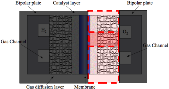
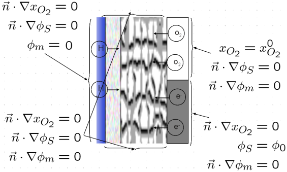
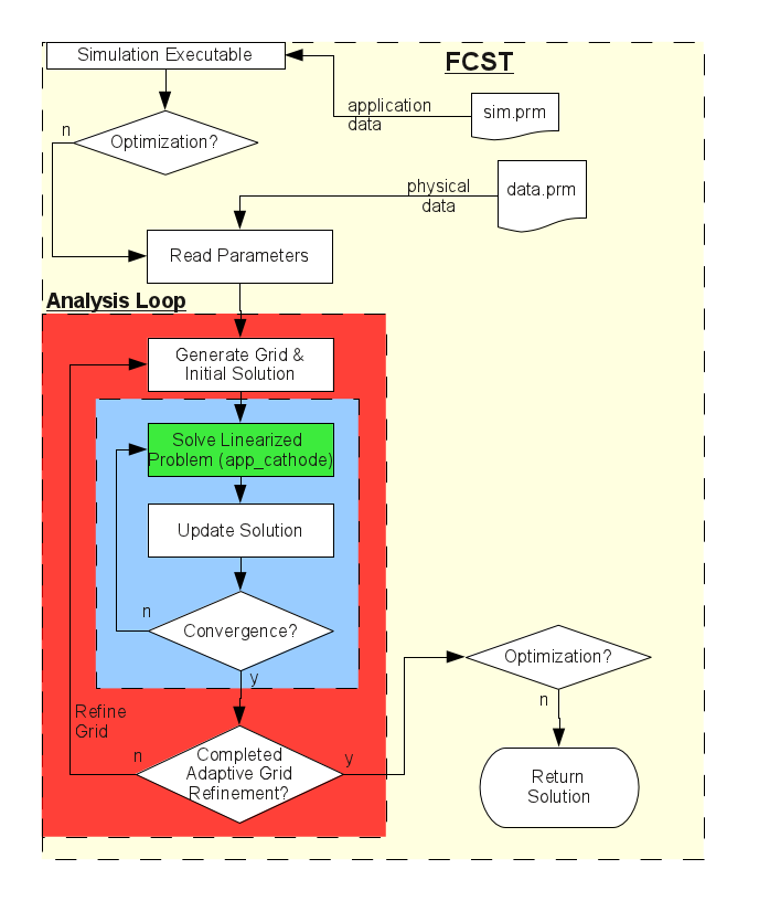
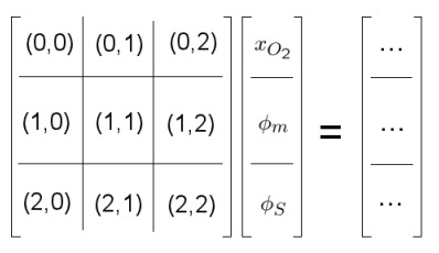
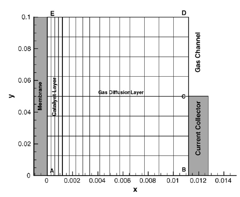
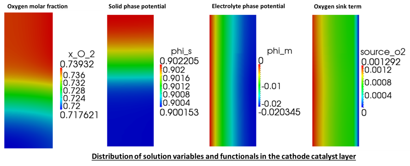

 1.8.2
1.8.2

